
模型已經能回應 API 請求,並不表示明天的預測仍然適用。資料來源可能換了欄位單位、使用者組成可能改變,真實標籤也可能幾週後才回來。服務沒有報錯,和模型仍然有用,是兩個問題。
上線後最容易犯的錯,是把所有問題壓成一個警報燈:drift 沒亮就說品質穩定,亮了就立刻重訓;總 accuracy 不錯,就以為各群體也都沒問題。
本篇用四個人工批次做兩個反例:分數分布完全相同,錯誤仍可增加;分數分布明顯改變,分類也可以繼續全對。讀者會親手跑出分布、錯誤與分群結果,再把它們接到標籤回補、調查與監控資料保存的判斷。
先問監控的問題,再選指標
一個預測系統有好幾種「有沒有變差」。至少要分清:
| 訊號 | 能回答的問題 | 還不能直接知道什麼 |
|---|---|---|
| 服務狀態 | 請求能否完成、錯誤率與延遲是否異常 | 預測是否符合真實結果 |
| 輸入/分數分布 | 跟參考期相比,觀察到的資料或輸出是否改變 | 改變是否造成品質下降 |
| 有可靠標籤後的品質 | 預測與實際結果的錯誤如何變化 | 每個未標註個案的真相、變化原因 |
| 分群與影響 | 錯誤是否集中在特定群體或情境 | 單一差距是否已證明歧視或公平 |
官方監控文件也會區分輸入特徵與輸出分布的監測。例如 Google 的監控概念頁 分別描述與訓練資料、過去服務資料比較的方式。這不表示本篇已啟動該服務,也不表示下面的四格 score histogram 就監控了所有原始特徵。
參考資料要跟問題一致。若拿訓練期當基準,問的是訓練與服務的差異;拿前一個成熟服務期,問的則是服務隨時間的變化。模型版本、前處理、資料量、時間窗口與切片定義都要留下來,否則比較兩條線之前,可能已換了計算對象。
儀表板也要看清楚目前選了什麼,不能只看見一排柱子就叫它 drift。
圖中 Diff w. baseline 顯示的是相對百分比。以 medium 為例,.68000 與 Overall .56183 的差約 .11817,換算為 11.817 個百分點;再除以 baseline,才是約 21.03% 的相對差:
絕對率差 = .68000 − .56183 ≈ .11817
相對差 = (.68000 − .56183) / .56183 ≈ 21.03%
先認出 metric、baseline、threshold 與單位,才知道自己在比較什麼。這張圖是來源文件的 UI 範例,未由本站執行,也不能把一個相對差直接當成品質、偏誤或法律判斷。
四個批次:分數分布不等於預測品質
原創程式每個批次都有 40 列,A、B 兩個人工 cohort 各 20 列。沒有訓練新模型,也沒有連上真實服務;score 與 label 都是為了拆解邏輯而手設。
參考批次每群都有 .2、.4、.6、.8 四種 score,各重複五次。分類閾值固定為 .5,score 大於或等於 .5 預測正類;前兩種 label 是 0,後兩種是 1,因此參考分類全對。
為比較分布,另外把 score 放進四格:
bin 0: [0, .25)
bin 1: [.25, .5)
bin 2: [.5, .75)
bin 3: [.75, 1]
注意分箱邊界與分類閾值是不同的設計。前者用來描述分布,後者用來做決策。參考 counts 是 [10,10,10,10],四格比例各 .25。
這裡用分箱後的 total variation distance 比較新批次 q 與參考 p:
TV = 0.5 × Σ_bins |p_bin − q_bin|
alert = TV > 0.2
.2 是教學手訂警報門檻,不是 p-value,也沒有透過抽樣變異校準誤報率。小批次波動、不同分箱與大量同時監測都會影響實際使用;本例沒有評估這些 detector 性能。
四個情境的實際輸出如下:
- 10/10/10/10
- 0
- 否
- 40
- 1
- 10/10/10/10
- 0
- 否
- 40
- .75
- 20/0/0/20
- .5
- 是
- 40
- 1
- 10/10/10/10
- 0
- 否
- 0
- null
第二列沒有任何 score 分布警報,卻真的多了十個錯誤。分數 marginal 相同,不能保證真實 label 跟分數的關係也相同;更不能保證所有原始特徵都不變。
第三列的 score 變得更靠近兩端,四格比例變成 [.5,0,0,.5],所以 TV=.5。但 score 仍在分類閾值正確的一側,accuracy 繼續為 1。這只是在固定 .5 決策下的反例,沒有比較 calibration 或證明模型所有品質都不變。
警報因此比較適合被讀成「這個觀察量值得調查」,而不是「模型一定壞了」。同樣地,沒有警報也只能說這種分箱、窗口與距離未超門檻,不能當成品質證書。
標籤延遲時,不能把不知道填成零
許多服務的真實結果不會跟預測一起出現。預測當下能記下 score,幾天後才知道結果;有些案例甚至一直沒有可靠回饋。
本例最後一個批次把 label 設為 None。score histogram 仍能計算,但 accuracy、confusion、TPR、FPR 都是 null。null 的意思是這裡沒有可用標籤來算,不是 accuracy=0,也不是 error=0。
標籤回來後,要配回當時的預測、模型版本與決策閾值,不能拿今天重新跑的模型冒充當時的預測。AWS 的品質監控文件 就明確描述以識別碼合併預測與 Ground Truth,且標籤收集日期可以晚於預測日期。本篇只採這個概念,未執行其雲端服務。
實務上還要記錄「哪段時間的預測已有多少標籤成熟」。例如最近一天只有容易取得的案例先回覆,直接跟上個月完整標籤的 accuracy 比,可能比較到回覆選擇差異。只對已知 label 算指標時,分母與標籤覆蓋率應一起報告,不能默認未回覆者跟已回覆者相同。
這支程式只示範全部已知與全部未知兩端,沒有實作延遲事件合併、選擇偏差修正或補標流程。回補不能靠猜 label 完成,更不應以模型自己的預測當 Ground Truth 來證明自己準。
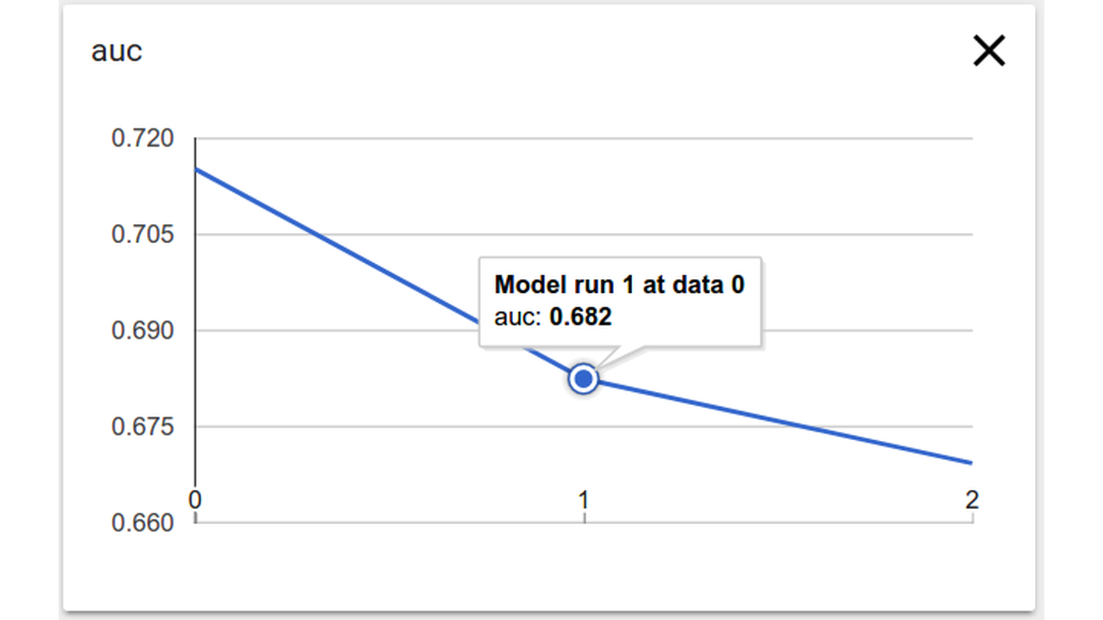
官方 TFMA basic 教學的相應段落會載入三個模型目錄、以同一份 data_location 評估,並明說 model-centric 圖的 X 軸是模型目錄名稱。要追時間趨勢,仍需另外核對每個點對應的模型、資料與時間窗口,不能只因折線向下,就猜測是某一天發生 drift。
看群體差距,先把分母攤開
在 score 相同、B labels 全改 0 的情境,總 accuracy=.75,A 為 1,B 為 .5。只看總平均,會漏掉錯誤集中在 B。
不過連「比較 TPR」也不能直接把兩個數字並排。這次實際 confusion 為:
- 10
- 10
- 20
- 0
- 1
- 1/3
- 10
- 0
- 10
- 0
- 1
- 0
- 0
- 10
- 10
- 0
- null
- .5
定義是:
TPR = TP / (TP + FN)  # 真實正類中,被判正的比例
FPR = FP / (FP + TN)  # 真實負類中,被判正的比例
B 這次沒有任何真實正類,TPR 的分母是零。寫成 0 會把「無法從這批資料估」偽裝成「真實正類一個也沒抓到」;寫成 1 同樣沒有依據。全局 TPR=1,也不表示每群 TPR 都能定義或都等於 1。
Fairlearn 的指標說明 區分選擇率與依 label 條件化的錯誤率,並提醒指標有其情境假設,切得越細也越容易遇到小樣本與多重比較問題。本例沒有採用一條差距門檻來宣布公平。
A、B 只是人工 cohort,不是實際人口或受保護屬性。把 B labels 改成全零,是刻意構造的數學案例,不是對真實群體的描述。實際偏誤調查還要看 label 是否可靠、錯誤造成什麼影響、誰沒有進入資料,以及群體定義是否適合問題;一個分群表不能直接推出歧視的原因或法律結論。
這三種率也不能看成同一個分母:balanced accuracy 在二元情境平均兩類 recall,FPR 以真實負類為分母,FNR 以真實正類為分母。把各群體拆開能發現平均掩蓋的差異,但仍要知道圖的資料與選擇過程。
這個來源範例特別加入由 Y 與 SEX 生成的半合成 Interest 欄位,並用 test metrics 參與 inner model 選擇。因此這張圖適合教「把多種率按群體攤開」,不能當未碰過的 holdout 證據、公平改善保證或真實金融部署建議。本文未重跑該教材;資料版本與改作歸屬另列於文末。
為了監控,要保存多少資料才夠?
監控需要紀錄,卻不表示每一筆原始請求都應永久完整保存。先列出調查目的,再決定欄位,比先收全量再想用途更容易控制範圍。
對分布與錯誤回補,本篇建議先分開思考三層:
| 用途 | 可能需要的紀錄 | 要另問的問題 |
|---|---|---|
| 日常趨勢 | 時間窗口、版本、樣本數、分箱計數、錯誤數 | 小樣本切片是否過細、誰能讀取? |
| label 回補 | 能配回當次預測的識別、預測時間/版本、回補狀態 | 識別碼如何控管,需保存多久? |
| 個案調查 | 經明確授權的必要欄位與有限樣本 | 能否用較少欄位,何時刪除,如何留存調查依據? |
這是設計討論,不是一份通用欄位清單。某個業務需要的回補資料,另一個業務可能完全不需要;刪掉識別碼若使回補無法進行,也要明確承認這個取捨。
NIST 2020 年的 Privacy Framework 1.0 在資料處理與 audit/log 管理中納入最小化、保留與刪除的考量,可作為這類工程討論的脈絡。它是風險管理框架,這裡沒有把它當成某地法規的合規判定。
彙總也不自動等於匿名。某些很小、可連結的切片仍可能暴露個人資訊;刪掉姓名不代表其他欄位不能連回同一個人。本例只有人工資料與計數,沒有實作差分隱私、去識別安全評估或隱私稽核。要保留多久、誰能存取與如何處理群體屬性,仍需依實際目的、風險與適用要求決定。
警報亮了,接下來是調查、限制還是回滾?
如果看到分布變化,先確認比較是否成立:窗口筆數是不是太少、時區或季節是否改變、某欄位是否換單位、前處理與模型是否剛換版?再看切片與成熟 label 的品質,有沒有真實影響或資料管線故障的證據。
回滾也要分清是哪一層。若新前處理把單位弄錯,修正管線可能比重訓更直接;若新模型在可比較成熟資料上出現不可接受的錯誤,可以依事先定義的責任與條件切回已保留版本。但若資料環境已改,舊模型也可能失效,不能因為它叫上一版,就假定比較安全。
較有用的處置紀錄會把「觀察到什麼、已知哪些影響、哪個版本與窗口、採取什麼措施、誰決定、何時重新檢查」連在一起。重大未知時也可能先限制自動化範圍或轉人工,而不是只在重訓/不重訓之間二選一。這些是依風險設計的判斷方向,本例沒有部署告警、回滾或人工覆核系統。
完整可執行程式:讓四個反例自己說話
原型使用 Python 標準函式庫,保存的實跑環境為 Python 3.10.12。把以下完整內容存成 monitor_batches.py,在同目錄執行:
python3 monitor_batches.py > stdout.json
成功時 exit 0,stdout 可解析成 JSON。四個 case 應分別得到前表的 counts/TV/accuracy;延遲標籤情境的 accuracy 與 confusion 為 null,B 無正類時的 TPR 也為 null。程式不訓練新模型、不寫監控資料庫,也不會真的送出告警。
輸入是這支程式自己產生的非空人工批次與合法 label,不是任意不可信資料的通用監控 API。重現這四個結果,不代表已驗過資料缺失、惡意輸入、抽樣波動或多重檢定。
"""Original constructed monitoring cases; not a calibrated detector or fairness/privacy guarantee."""
import json


def make_batch(scores=(.2, .4, .6, .8), change_b_labels=False, labels_available=True):
    rows = []
    for group in ("A", "B"):
        for _ in range(5):
            for i, score in enumerate(scores):
                label = int(i >= 2)
                if change_b_labels and group == "B":
                    label = 0
                rows.append({"group": group, "score": score,
                             "label": label if labels_available else None})
    return rows


def distribution(rows):
    # Fixed, left-closed bins [0,.25), [.25,.5), [.5,.75), [.75,1].
    counts = [0, 0, 0, 0]
    for row in rows:
        score = row["score"]
        if not 0 <= score <= 1:
            raise ValueError("Score outside [0,1]")
        counts[min(int(score * 4), 3)] += 1
    return {"counts": counts, "proportions": [n / len(rows) for n in counts]}


def labeled_metrics(rows):
    known = [r for r in rows if r["label"] is not None]
    if not known:
        return {"total": len(rows), "labeled": 0, "accuracy": None,
                "confusion": None, "TPR": None, "FPR": None}
    tp = sum(r["label"] == 1 and r["score"] >= .5 for r in known)
    fp = sum(r["label"] == 0 and r["score"] >= .5 for r in known)
    tn = sum(r["label"] == 0 and r["score"] < .5 for r in known)
    fn = sum(r["label"] == 1 and r["score"] < .5 for r in known)
    return {"total": len(rows), "labeled": len(known), "accuracy": (tp + tn) / len(known),
            "confusion": {"TP": tp, "FP": fp, "TN": tn, "FN": fn},
            "TPR": tp / (tp + fn) if tp + fn else None,
            "FPR": fp / (fp + tn) if fp + tn else None}


def describe(rows, reference_distribution):
    actual = distribution(rows)
    tv = .5 * sum(abs(a - b) for a, b in zip(actual["proportions"], reference_distribution["proportions"]))
    return {"score_distribution": actual, "score_histogram_total_variation": tv,
            "handset_threshold": .2, "histogram_alert": tv > .2,
            "all": labeled_metrics(rows),
            "groups": {g: labeled_metrics([r for r in rows if r["group"] == g]) for g in ("A", "B")}}


def main():
    reference = make_batch()
    reference_distribution = distribution(reference)
    cases = {"reference": describe(reference, reference_distribution),
        "same_scores_changed_B_labels": describe(make_batch(change_b_labels=True), reference_distribution),
        "shifted_scores_same_correct_decisions": describe(make_batch(scores=(.05, .1, .9, .95)), reference_distribution),
        "same_scores_labels_delayed": describe(make_batch(change_b_labels=True, labels_available=False), reference_distribution)}
    assert cases["reference"]["all"]["accuracy"] == 1
    changed = cases["same_scores_changed_B_labels"]
    assert changed["score_histogram_total_variation"] == 0 and not changed["histogram_alert"]
    assert changed["all"]["accuracy"] == .75
    assert changed["groups"]["A"]["accuracy"] == 1 and changed["groups"]["B"]["accuracy"] == .5
    assert changed["groups"]["B"]["TPR"] is None and changed["groups"]["B"]["FPR"] == .5
    shifted = cases["shifted_scores_same_correct_decisions"]
    assert shifted["score_histogram_total_variation"] == .5 and shifted["histogram_alert"]
    assert shifted["all"]["accuracy"] == 1
    assert cases["same_scores_labels_delayed"]["all"]["accuracy"] is None
    print(json.dumps({"scope": "Four constructed 40-row batches, fixed score threshold .5, no model training or live monitor",
        "cases": cases,
        "limits": ["Histogram drift is score-distribution drift only, not all raw features or all concept changes.",
            "Threshold .2 is hand chosen, not calibrated for sampling noise, false alarms or multiple tests.",
            "Labels are changed by construction; real shifts require investigation and trustworthy feedback.",
            "A/B are synthetic cohorts, not actual protected demographics or proof of fairness/unfairness.",
            "Undefined rates are null, not zero; missing labels do not authorize reporting accuracy.",
            "Aggregate counts alone do not establish anonymity, privacy compliance or differential privacy.",
            "No latency/load, alert service, privacy audit or production outcome was measured."]}, indent=2, allow_nan=False))


if __name__ == "__main__":
    main()
上線後最有價值的監控,會把尚不知道的事也保留下來:分數變了但品質未明,label 未成熟所以指標不能算,某群沒有正類所以 TPR 無法估。能把訊號、分母與未知分開,才有足夠依據決定下一個調查與處置。
來源與延伸閱讀:
-
Google Model Monitoring 概念:採分布與參考資料的角色;查閱的是當前頁面,未把新產品功能回填成 2023 年以前的歷史。本文未使用其服務或距離實作。
-
AWS Ground Truth 與預測合併:可靠 label 與預測配對;本文未啟動雲端監控。
-
Fairlearn 常見公平性指標:群體率的條件與情境限制。該 URL 頁首標示 0.11.0.dev0,本文只採公式概念,沒有宣稱安裝或執行某個 Fairlearn 版本。
-
NIST Privacy Framework 1.0,2020:CT.PO-P2、CT.DM-P 與 CT.DM-P8 的保留/刪除及 log 最小化脈絡;不是特定司法管轄區法律建議或本例合規證書。
-
圖 1:TensorFlow Fairness Indicators;圖 2:TFMA Visualizations 與 TFMA basic 的 Tracking Model Performance Over Time。頁面文件內容的 CC BY 4.0 與 code 的 Apache grant 分開;本篇採文件自有示意截圖,未執行其服務。
-
圖 3:Fairlearn Credit Loan Decisions、固定原始程式 與 MIT 授權。本文只用來源圖解讀分群指標,不搬用其 test 選模作本例驗收方式。
-
圖 3 資料:I-Cheng Yeh(2009),Default of Credit Card Clients,UCI,DOI 10.24432/C55S3H,CC BY 4.0。Fairlearn 已刪改/重新命名欄位並加入半合成 Interest;本文沒有重散布原始資料列。
圖像來源、資料署名與完整授權聲明:
DS71 image sources and modifications

Figures 1–2 and cover: TensorFlow documentation authors, Fairness Indicators (https://www.tensorflow.org/tfx/guide/fairness_indicators) and TensorFlow Model Analysis Visualizations (https://www.tensorflow.org/tfx/model_analysis/visualizations). The source pages license their documentation content under CC BY 4.0 (https://creativecommons.org/licenses/by/4.0/), except where otherwise noted. These selected images are the pages' own documentation screenshots, not code samples. Main files are reproduced unchanged. The mobile view of Figure 1 preserves the whole screenshot first and repeats its complete right metric panel at larger size, using source pixels only. The cover fits the whole Figure 2 chart proportionally on a white canvas. No data, labels or plot marks are added or changed. The height slices and the three-point AUC graph are documentation examples, not this project's synthetic batch results, a score-drift detector, or proof of fairness.

Figure 3: Microsoft Corporation and Fairlearn contributors, Credit Loan Decisions, Fairlearn 0.12.0, https://fairlearn.org/v0.12/auto_examples/plot_credit_loan_decisions.html . Pinned source: https://github.com/fairlearn/fairlearn/blob/aeac30d6b1adcff7d24e6af69990ca1552b81210/examples/plot_credit_loan_decisions.py . Figure 008 is the ExponentiatedGradient selected inner-model group-metrics chart (epsilon=.01, index=14), in the section Selecting a suitable inner model, after the earlier separate ThresholdOptimizer section. It is not ThresholdOptimizer output. The original main PNG is unchanged; the mobile version preserves the complete original first and then repeats the three original metric panels in order at larger size. Only source-pixel crops and proportional resizing/white spacing are used, without relabeling or changing plotted data.

Data credit for Figure 3: I-Cheng Yeh (2009), Default of Credit Card Clients, UCI Machine Learning Repository, https://doi.org/10.24432/C55S3H and https://archive.ics.uci.edu/dataset/350/default+of+credit+card+clients , CC BY 4.0 (https://creativecommons.org/licenses/by/4.0/). The Fairlearn example drops/renames fields and adds a semi-synthetic Interest feature generated from Y and SEX to construct a teaching disparity. It also uses test-set metrics when selecting the inner model; the displayed metrics are not untouched-holdout evidence, this project's results, a representative population finding, or a production lending recommendation. No original dataset records are redistributed in this article.

Fairlearn original MIT License (verbatim)
    MIT License

    Copyright (c) Microsoft Corporation and Fairlearn contributors.

    Permission is hereby granted, free of charge, to any person obtaining a copy
    of this software and associated documentation files (the "Software"), to deal
    in the Software without restriction, including without limitation the rights
    to use, copy, modify, merge, publish, distribute, sublicense, and/or sell
    copies of the Software, and to permit persons to whom the Software is
    furnished to do so, subject to the following conditions:

    The above copyright notice and this permission notice shall be included in all
    copies or substantial portions of the Software.

    THE SOFTWARE IS PROVIDED "AS IS", WITHOUT WARRANTY OF ANY KIND, EXPRESS OR
    IMPLIED, INCLUDING BUT NOT LIMITED TO THE WARRANTIES OF MERCHANTABILITY,
    FITNESS FOR A PARTICULAR PURPOSE AND NONINFRINGEMENT. IN NO EVENT SHALL THE
    AUTHORS OR COPYRIGHT HOLDERS BE LIABLE FOR ANY CLAIM, DAMAGES OR OTHER
    LIABILITY, WHETHER IN AN ACTION OF CONTRACT, TORT OR OTHERWISE, ARISING FROM,
    OUT OF OR IN CONNECTION WITH THE SOFTWARE OR THE USE OR OTHER DEALINGS IN THE
    SOFTWARE
留言0
登入後就能留言。
登入