
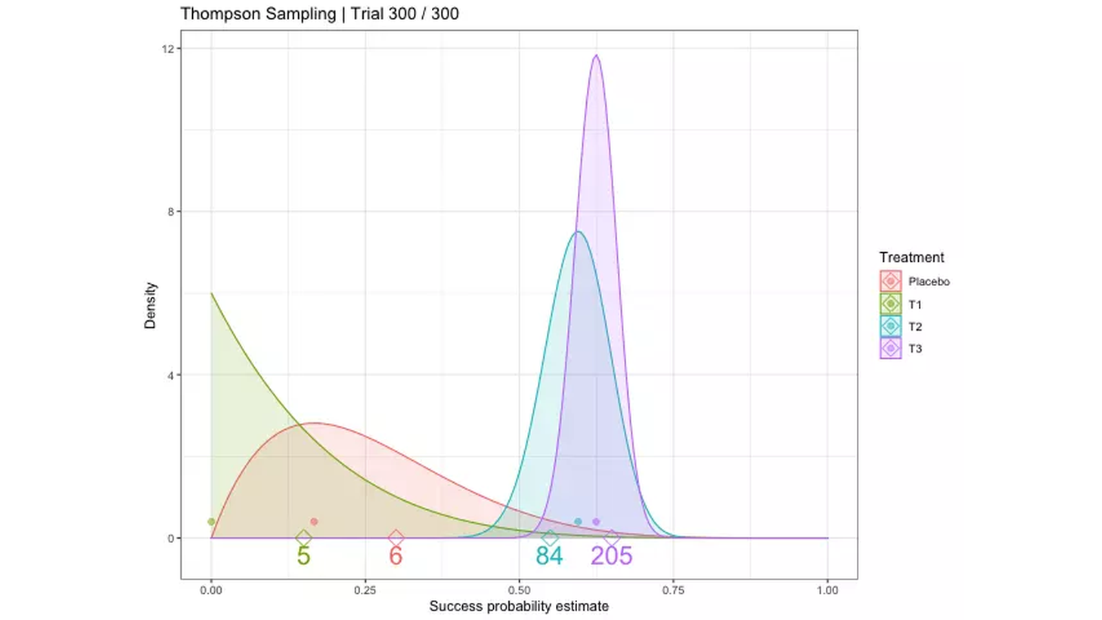
你有三種推薦版位、三個標題,或三個可以展示的候選方案。每次只能挑一個,然後看到這次是否成功。你看不到同一個人、同一個時刻,換成另外兩個選項會發生什麼。
如果一直選目前成功率最高的方案,可能把早期運氣誤認成實力;如果永遠平均分配,又會把很多機會花在已經知道比較差的選項。Multi-Armed Bandit,通常簡稱 bandit,研究的正是這種邊做決定、邊蒐集資訊的問題。
本篇從只有三個選項、獎勵為 0 或 1 的例子出發,拆解 greedy、ε-greedy、UCB 與 Thompson Sampling。完整標準庫程式會實際模擬五種策略,但重點是看懂每個策略知道什麼、如何更新,以及「拿到多少獎勵」與「選擇損失了多少期望值」為何是兩件事。
關鍵不是三根拉桿,而是只看得到選中的回饋
上一篇 BPR 排序從既有互動構造相對偏好。Bandit 再往前一步:策略本身會影響接下來收集到什麼資料。選了 A,就收到 A 的回饋;沒有選 B、C,這次就沒有它們的結果可用。
最簡單的 stationary bandit 假設每個選項,也叫一個 arm,都有固定的獎勵分布。每次選一臂,立刻拿到它的獎勵。策略希望在有限的 T 次選擇裡,累積盡量多的獎勵,而不是只把最後一次成功率估得準。
本篇程式的三臂真實成功率為:
arm 0:μ₀ = 0.20
arm 1:μ₁ = 0.50
arm 2:μ₂ = 0.65
每次 reward 為 0 或 1;總共 T = 200 次選擇。
這三個 μ 是模擬環境的設定。評分者知道它們,所以可以檢查策略付出了多少機會成本;策略不能讀 μ,也不能偷看未選臂的獎勵,只能從自己的已選回饋更新。
先看來源圖中的叉號與菱形:少量樣本的平均可以遠離真實均值。這是早期一直利用同一選項的風險。圖上菱形只是讓讀者看得見的模擬真值,不代表實際策略能讀到答案;本篇程式同樣把真值留給環境和評估。
這個問題還有幾個重要簡化:沒有使用者特徵、成功立刻回報、三臂成功率不隨時間改變,也沒有一次選擇改變下一個使用者狀態的機制。這些前提讓我們能先看清探索與利用;真實推薦是否符合,還需要另行判斷。
Greedy 為什麼會卡住?ε-greedy 多給哪些機會?
對一臂最直接的估計,是把觀察到的成功次數除以拉臂次數:
目前平均 Q(a) = successes(a) / counts(a)
Greedy 每次都選目前平均最高的一臂。假如某個較好的方案第一次剛好失敗,平均就變成 0;另一個普通方案剛好成功,平均變成 1。Greedy 可能一直選後者,使前者沒有足夠新資料翻身。它是在利用現有估計,不是每次都選真正最好的方案。
為了讓所有策略起點清楚,本例先固定各拉臂一次:第 1、2、3 次依序拉 0、1、2,這三次也算在 T=200 裡。之後 greedy 只比較樣本平均,同分選較小 ID。這能避免完全沒拉過的臂沒有分母,卻不能保證一次觀察就夠。
ε-greedy 加了一條簡單分支:大部分時間照 greedy,少部分時間不看目前平均,均勻隨機選一臂。本篇固定 ε=.1:
90% 的決策:選目前平均最高的一臂
10% 的決策:從全部三臂均勻抽一臂
隨機分支也可能抽中 greedy 臂。假如目前只有一個最大平均,它被選中的總機率是 .9+.1/3=.933333…;兩個非 greedy 臂各有 .1/3 的機會。因此 ε=.1 不能直接翻成「10% 的時間一定選較差的臂」。
這種探索不需判斷哪一臂最值得補資料,容易實作,但也因此不分青紅皂白:很接近最佳、仍不確定的臂,和明顯較差的臂,都可能得到相同的隨機機會。固定 ε 還會持續付出探索成本;跑得更久、差距不同,或成功率開始漂移,都可能改變適合的策略和參數。
UCB:平均相近時,把不確定性放進選擇
UCB 的想法不是只問目前平均誰最高,而是把「平均還不確定」也納入指標。對 Auer 等人的 UCB1,本文使用:
index(a) = Q(a) + sqrt(2 × ln(t) / n(a))
選 index 最大者;同分選較小 ID。

t:目前已完成的總拉臂次數
n(a):其中選過臂 a 的次數
這裡 t 的定義很重要:前三次初始化完成後,準備做第 4 次決策時,t=3,各臂 n=1。這沿原論文演算法框的 completed-plays 記號,沒有把「第幾次決策」和「已完成幾次」混成同一個數字。前三次已保證各臂拉過一次,所以不會除以 0。
補償項可以直接拆開讀:n(a) 大,代表這臂看過較多次,補償變小;一直不選某臂時,它的 n 不增加,但總時間 t 增加,補償就可能變大,促使策略回頭看它。這是一種樂觀探索,並不是向環境索取未選臂的真實結果。
UCB1 的 index 可能超過 1。即使獎勵是 0/1,也不表示這個 index 應當解讀成點擊機率;它是平均加探索補償,用來比較選擇。把它強制截到 1,已經改了原策略。
UCB 有帶條件的理論分析,例如 stationary、獨立且落在 [0,1] 的獎勵。這些條件符合本例的環境設計,但不表示 20 個種子的短模擬必須讓 UCB 排第一,也不表示每條單次獎勵路徑都符合平均遺憾上界的曲線形狀。當回饋延遲、成功率漂移或同一使用者反覆出現時,不能直接拿這個最簡版本的結論代替實驗。
Thompson Sampling:抽一套可能的成功率,再選最好的一臂
ε-greedy 的隨機性來自「有時任意抽臂」;Thompson Sampling 的隨機性來自「對未知成功率的後驗分布抽樣」。本篇用最容易手算的 Beta–Bernoulli 配對。
每臂的 reward 為 0/1,先驗設成 Beta(1,1),也就是 [0,1] 上的均勻分布。看見一次成功,該臂 alpha 加 1;看見一次失敗,beta 加 1:
posterior(a) = Beta(1 + successes(a), 1 + failures(a))

每次決策:
1. 每臂各抽一個可能成功率 θ̃(a)
2. 選抽到的 θ̃ 最大的一臂
3. 只用該臂這次的 0/1 回饋更新它
抽到的 .7 是「這臂成功率可能為 .7」的一個樣本,不是預先知道這次一定成功,也不是在 policy 裡先替全部臂製造反事實點擊。真正的當次 reward 仍要選完之後,由環境回傳。
例如本例某臂先後得到 1、0、1,後驗就是 Beta(3,2),平均為 3/5=.6。這個平均不等於策略每次一定拿 .6 去比較;Thompson 每次仍重新抽樣。另一臂即使平均稍低,只要不確定性使它仍有機會是最佳,抽樣就可能給它探索機會。
後驗密度高不等於「這臂成功率超過 100%」。密度曲線的高度可以大於 1,整段區域的面積才對應機率。圖中後期變窄變高,表達的是對成功率的不確定性縮小。
Thompson 的信念也依賴模型前提。獨立 Beta 先驗、固定成功率、立刻看到成功或失敗,是這個簡單版本的合約。它沒有替不同使用者建模,也不會自動處理成功幾天後才發生、某些失敗被漏記,或介面改版後成功率突然變動。
把比較做成可檢查的實驗,而不是看一條順眼曲線
本篇三臂環境與上面的兩位圖像作者設定不同。五種策略都用同一組真實成功率 [.2,.5,.65],每個 seed 各做 200 次決策,包含前三次固定拉臂。共 20 個 seed,合計 5×20=100 runs、20000 次決策。
如何讓比較可以重跑?每個 seed 先產生一張「全域時間×臂」的潛在 reward 表:200 列、每列三個獨立 Bernoulli 值。五種策略共用同一張表,同一時間選同一臂就收到同一格;如果它們選不同臂,自然讀不同格。
這是模擬者為比較而固定的環境,不是策略獲得額外資訊。程式先讓 choose() 只看自己的 counts、successes 與策略 RNG,選完後,才把表中選中的那一格交給 observe()。未選中的格沒有交給策略。環境 RNG 與 policy RNG 分開,策略多抽幾次隨機數不會讓環境換一張表。
還要分清另一種常見耦合方式:本篇不是「第 n 次拉某臂,永遠讀該臂第 n 個 reward」。這裡索引是全域時間;同一臂如果在不同時間被選,讀的也可能是不同格。兩者都可以用來設計模擬,但比較規則必須先說明。
Greedy 用樣本平均,並不是另一種用 Beta 後驗平均的 Bayesian greedy。TS 加了共同的三次 warm start,也不是宣稱所有 TS 實作都要強制先拉每臂一次。這些選擇沒有拿本次結果調參;20 個種子改的是觀察與策略隨機性,沒有產生 20 種不同成功率問題。
累計獎勵、pseudo-regret 與 realized gap 要分開
累計 reward 最容易看懂:200 次裡一共成功幾次。但比較探索成本時,模擬評分者還能利用真實 μ,計算這條選擇路徑付出了多少期望值:
最佳真實均值 μ* = 0.65
pseudo-regret = Σ_t (μ* − μ[選中的臂])
             = 0.45 × count(arm0) + 0.15 × count(arm1)
每一項都非負。選最佳臂 2,該次的 mean gap 為 0;選臂 0,就記 .45。不論這一次運氣好不好、reward 是 0 還是 1,這個 gap 都是由所選臂的真實均值決定。
另一個容易被混稱 regret 的量,是用最佳臂的期望總 reward 減去實際拿到的 reward:
realized gap = T × μ* − observed cumulative reward
             = 130 − observed cumulative reward
這個量可以是負的。保存結果裡,seed 14 的 greedy 成功了 142 次,所以 realized gap=−12。這不表示它找到比 .65 更好的真實臂,也不是 pseudo-regret 變成負數;只是這一條隨機獎勵路徑超過了 130 這個期望基準。
若在此固定 stationary 合約下對所有環境與策略隨機性取期望,realized gap 和路徑 pseudo-regret 的期望對應。單次數字不同,有限 20 個種子的平均也不必剛好相等。真實服務不知道各臂 μ,不能直接從一次點擊紀錄算出同樣的 oracle pseudo-regret。
實際運行得到以下 20-seed 算術平均:
| 策略 | 累計 reward | Pseudo-regret | Realized gap |
|---|---|---|---|
| Random | 92.30 | 38.3775 | 37.70 |
| Greedy | 114.00 | 17.3025 | 16.00 |
| ε=.1 | 119.10 | 12.7800 | 10.90 |
| UCB1 | 115.80 | 16.5375 | 14.20 |
| Thompson Beta | 120.25 | 11.5575 | 9.75 |
在這批設定裡,TS 的平均 reward 較多、pseudo-regret 較小;UCB1 也沒有贏過 ε=.1。這些結果照實保留,但不是通用演算法排名:horizon、成功率差距、初始化、隨機種子與探索參數都會影響數字。本文沒有做顯著性檢定、參數搜尋或真實線上 lift 實驗。
完整 JSON 還保留每個 seed/policy 的 arm counts、successes、三種總量和平均,以及 seed 0 的完整已選回饋軌跡。這讓你可以從 counts 重算 pseudo-regret,再從 successes 合計核對 reward,而不必只相信最後的 summary 表。
用標準庫重跑:檢查資訊流和更新,不只對照平均值
實際執行環境為 Python 3.10.12、CPU,只用 Python 標準庫,沒有第三方套件。把下方完整程式存成 bernoulli_bandit_policies.py,在同目錄執行:
python3 bernoulli_bandit_policies.py > stdout.json
對應的 requirements.txt 只有環境說明,不需要 pip 安裝套件:
# Python 3.10.12; standard library only. No third-party packages required.
成功時 exit 0,產生可解析的 JSON。請先查每組 arm counts 合計為 200、reward 等於 successes 合計,seed 0 的前 3 個動作皆為 [0,1,2];再確認 policy 只在選完後收到一個 binary reward。檔案裡也列出每個 seed 的潛在表 hash,便於對照同一環境。
同一記錄版本下的 beta 抽樣可重現本次結果;沒有承諾所有 Python 實作與版本的隨機抽樣都逐 byte 相同。這份程式也沒有對外部動態臂、非二元 reward 或延遲回饋提供通用服務介面。
"""Original stationary, immediate-feedback Bernoulli bandit mechanics.

Only the environment/evaluator knows the true means and potential outcomes.
Every policy sees just its own chosen-action feedback. No contextual features.
"""
import hashlib
import json
import math
import platform
import random


MEANS = (0.2, 0.5, 0.65)
HORIZON = 200
SEEDS = tuple(range(20))
EPSILON = 0.1
POLICIES = ("random", "greedy", "epsilon_0_1", "ucb1", "thompson_beta")


def argmax_low_id(values):
    """Python max keeps the first ID when values are equal."""
    return max(range(len(values)), key=lambda arm: values[arm])


class Policy:
    """No true means, unchosen rewards or environment RNG are passed here."""
    def __init__(self, name, number_of_arms, seed):
        self.name = name
        self.rng = random.Random(seed)
        self.counts = [0] * number_of_arms
        self.successes = [0] * number_of_arms

    def choose(self):
        completed = sum(self.counts)
        number_of_arms = len(self.counts)
        # All policies share this explicit warm start, included in HORIZON.
        if completed < number_of_arms:
            return completed
        if self.name == "random":
            return self.rng.randrange(number_of_arms)
        averages = [s / n for s, n in zip(self.successes, self.counts)]
        if self.name == "greedy":
            return argmax_low_id(averages)
        if self.name == "epsilon_0_1":
            if self.rng.random() < EPSILON:
                # Exploration samples ALL arms, so it may select the greedy arm.
                return self.rng.randrange(number_of_arms)
            return argmax_low_id(averages)
        if self.name == "ucb1":
            # t is completed plays; first post-warm-start decision uses t=3.
            indexes = [q + math.sqrt(2 * math.log(completed) / n)
                       for q, n in zip(averages, self.counts)]
            return argmax_low_id(indexes)
        if self.name == "thompson_beta":
            # Beta(1,1) prior: successes -> alpha; failures -> beta.
            draws = [self.rng.betavariate(1 + s, 1 + n - s)
                     for s, n in zip(self.successes, self.counts)]
            return argmax_low_id(draws)
        raise ValueError("Unknown policy")

    def observe(self, arm, reward):
        if reward not in (0, 1):
            raise ValueError("This prototype accepts binary rewards only")
        self.counts[arm] += 1
        self.successes[arm] += reward


def potential_rewards(seed):
    """Independent time x arm Bernoulli cells; shared across policies per seed."""
    environment_rng = random.Random(seed)
    return [[int(environment_rng.random() < mean) for mean in MEANS]
            for _ in range(HORIZON)]


def run_policy(name, policy_seed, table):
    policy = Policy(name, len(table[0]), policy_seed)
    actions, rewards = [], []
    for time_index, row in enumerate(table):
        action = policy.choose()
        # The policy never receives row, including unchosen potential rewards.
        reward = row[action]
        policy.observe(action, reward)
        actions.append(action)
        rewards.append(reward)
    assert actions[:3] == [0, 1, 2]
    assert sum(policy.counts) == HORIZON
    assert sum(policy.successes) == sum(rewards)
    return policy, actions, rewards


def main():
    records = []
    trace_seed_zero = {}
    table_hashes = []
    best_mean = max(MEANS)
    for seed in SEEDS:
        table = potential_rewards(seed)
        payload = json.dumps(table, separators=(",", ":")).encode("ascii")
        table_hashes.append({"seed": seed, "sha256": hashlib.sha256(payload).hexdigest()})
        for policy_id, name in enumerate(POLICIES):
            policy_seed = 10000 + seed * 100 + policy_id
            policy, actions, rewards = run_policy(name, policy_seed, table)
            total_reward = sum(rewards)
            pseudo_regret = math.fsum((best_mean - mean) * count
                                     for mean, count in zip(MEANS, policy.counts))
            # This random realized gap is NOT the sum of nonnegative mean gaps.
            realized_gap = HORIZON * best_mean - total_reward
            assert math.isclose(pseudo_regret,
                                math.fsum(best_mean - MEANS[a] for a in actions), abs_tol=1e-12)
            records.append({"seed": seed, "policy": name, "policy_rng_seed": policy_seed,
                "cumulative_reward": total_reward,
                "pseudo_regret": round(pseudo_regret, 12),
                "realized_gap_to_best_expected_total": round(realized_gap, 12),
                "arm_counts": policy.counts, "arm_successes": policy.successes,
                "empirical_means": [round(s / n, 12) for s, n in zip(policy.successes, policy.counts)]})
            if seed == 0:
                trace_seed_zero[name] = {"actions": actions, "observed_rewards": rewards}
    metric_names = ("cumulative_reward", "pseudo_regret", "realized_gap_to_best_expected_total")
    summary = {}
    for name in POLICIES:
        rows = [row for row in records if row["policy"] == name]
        summary[name] = {"number_of_seeds": len(rows), **{
            "mean_" + metric: round(math.fsum(row[metric] for row in rows) / len(rows), 12)
            for metric in metric_names},
            "mean_arm_counts": [round(math.fsum(row["arm_counts"][a] for row in rows) / len(rows), 12)
                                for a in range(len(MEANS))]}
    print(json.dumps({
        "scope": "Fixed stationary Bernoulli means, no context, immediate chosen-action feedback; "
                 "original simulation, not an online recommendation experiment or universal policy ranking.",
        "versions": {"python": platform.python_version(), "dependencies": "Python standard library only"},
        "settings": {"true_means_for_environment_and_evaluation_only": MEANS,
            "horizon_including_three_warm_start_pulls": HORIZON, "seeds": SEEDS,
            "policies": POLICIES, "epsilon": EPSILON,
            "ucb1": "empirical_mean + sqrt(2*ln(completed_plays)/arm_count), completed_plays=3 at round4",
            "thompson": "independent Beta(1,1) priors; posterior Beta(1+successes,1+failures)",
            "warm_start": "Each policy chooses arms0,1,2 at global time indices0,1,2, included in T=200",
            "tie_break": "lowest arm ID for equal indexes or equal sampled values",
            "environment_seed": "random.Random(seed)",
            "policy_seed": "random.Random(10000 + seed*100 + fixed_policy_id)",
            "coupling": "Same full global-time-by-arm potential-reward table per seed for all policies; "
                        "not indexed by the number of times an arm has been pulled"},
        "metric_definitions": {
            "cumulative_reward": "sum of observed selected-cell rewards",
            "pseudo_regret": "sum_t (max(mu)-mu[action_t]); nonnegative for each chosen-action path",
            "realized_gap_to_best_expected_total": "T*max(mu)-observed_reward; may be negative; "
                                                   "not regret against a realized clairvoyant reward sequence",
            "summary": "arithmetic means over the same20fixed-environment seeds; not significance tests"},
        "per_seed_records": records, "summary": summary,
        "seed_zero_full_chosen_feedback_traces": trace_seed_zero,
        "potential_table_sha256": table_hashes,
        "limits": ["All policies use only their own past chosen-action counts and binary feedback.",
            "True means and unchosen cells are evaluator information, unavailable to choose().",
            "All policies receive an identical3pull warm start; this differs from TS with no forced initialization.",
            "Greedy uses empirical means, not the Beta posterior means of a Bayesian greedy policy.",
            "Exploration can reselect the greedy action; epsilon is not the probability of a nongreedy action.",
            "Fixed epsilon.1 and UCB1 coefficient were not tuned using these results.",
            "The twenty seeds vary outcomes/policy randomization, not the underlying mean vector.",
            "No nonstationarity, delayed/censored feedback, user heterogeneity, exposure correction or actual lift.",
            "A finite realized simulation need not order policies as a regret theorem or a longer run would.",
            "Reproduction of beta draws is scoped to the recorded Python implementation/version."]}, indent=2))


if __name__ == "__main__":
    main()
什麼時候這個簡單問題已經不夠?
如果成功率會隨時間變化,累積到很久以前的平均可能反而拖慢反應;如果每個使用者不同,就需要把情境和行動的關係納入,而不是追一個所有人共用的最佳臂。這些已經離開本篇 stationary、無 context 的合約。
還有更根本的差別:某次選擇若會改變接下來的狀態,例如使用者疲勞、長期留存或內容供應,本次只最大化即時 0/1 獎勵的模型未必服務真正目標。不能因為有探索,就把它等同完整的長期強化學習問題。
Bandit 讓資料蒐集策略成為模型的一部分,也讓你必須正視「沒有選就沒有回饋」。從這裡出發,先說清獎勵、可用行動、資訊可見性與時間前提,再決定探索方式。比起直接套一個漂亮策略名稱,這些定義更能決定後面的數字是否回答了你真正的問題。
來源與延伸閱讀:
- Sutton、Barto,Reinforcement Learning: An Introduction,第二版作者頁,第 2 章:sample-average、探索與利用、ε-greedy、UCB 與 contextual bandit 的區分。書中 10-arm Gaussian testbed 不是本文的 Bernoulli 設定;書籍圖片未重刊。
- Auer、Cesa-Bianchi、Fischer(2002),Finite-time Analysis of the Multiarmed Bandit Problem,原論文保存 PDF。本文 UCB1 的初始化與 completed-plays index 依原演算法;沒有重刊其論文圖。
- Russo、Van Roy、Kazerouni、Osband、Wen(2018),A Tutorial on Thompson Sampling,作者 PDF,§3 Beta–Bernoulli 與 Algorithm 2;arXiv。抽取後驗成功率與更新所選臂的機制由此支持;未重刊教材圖。
- Adrien PREVOST,UCB-type run,2026 自有視覺示意,CC0 1.0。抽取原影格只協助讀機制,並非 2002 原論文結果或本站實驗。
- Nguiard,Example of Thompson sampling,2020 自有模擬動畫,CC BY 4.0。原影格整體保留、依序直排,不新增曲線或臨床結論。
圖像來源與改作聲明:
Image source attribution and changes (selected illustrations)

Fig. 1, 2 and 5 — “UCB-type run.gif” by Adrien PREVOST, https://commons.wikimedia.org/wiki/File:UCB-type_run.gif, dedicated to the public domain under CC0 1.0: https://creativecommons.org/publicdomain/zero/1.0/ . The figures show complete source frames 0, 50 and 196 (zero-based). The selected frames were decoded from the original 560×800 animation and alpha-composited on white as PNGs. No plot content was cropped, redrawn, or changed. The original file is labelled “UCB-type”; no exact algorithm variant, parameterization, code, or seed is provided, so these images should not be attributed to canonical UCB1 or a repeated-run benchmark. In frame 196 the displayed arm counts are 173, 15 and 13 (sum 201) while the source x-axis tick extent reaches 200; the source has not been altered and the frame index is not presented as a round number.

Fig. 3, 4 and cover — “Example of Thompson sampling.webp” by Nguiard, https://commons.wikimedia.org/wiki/File:Example_of_Thompson_sampling.webp, licensed under CC BY 4.0: https://creativecommons.org/licenses/by/4.0/ . The original 640×480 animation is a simplified simulated treatment-efficacy illustration, not clinical evidence. Figures 3 and 4 use complete zero-based frames 0/20 and 100/300, respectively, stacked in source order with a 24-pixel white separator. The cover uses complete frame 300 scaled proportionally to 1200×900 and centered on a white 1600×900 canvas. These are frame extractions/layout derivatives; no plotted labels, values, curves, or data were redrawn or changed. Frame 0 shows four overlapping uniform density-1 priors with zero pulls, rather than an empty plot. In frame 100, legend-order Placebo/T1/T2/T3 counts are 3/4/25/68; in frame 300 they are 6/5/84/205. Count order follows the source legend, not the left-to-right colored marks.

The UCB and Thompson sampling images come from two separate source simulations and should not be compared as a shared experiment. All published use remains subject to the linked source licenses and accurate attribution.
留言0
登入後就能留言。
登入