
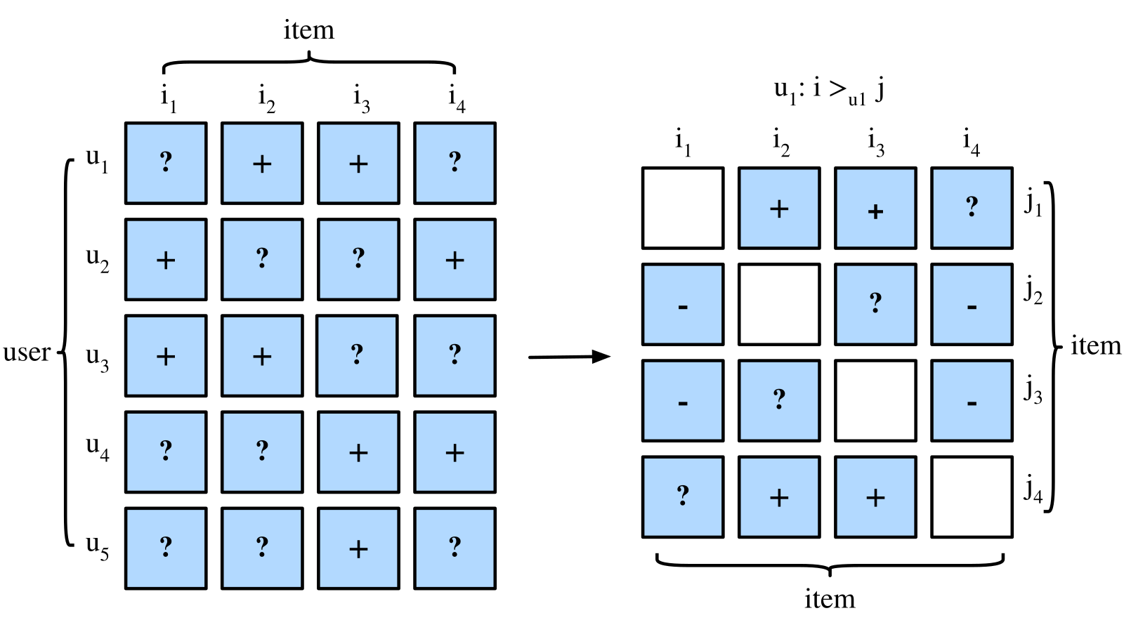
使用者點了 A,沒有點 B。你能因此替 A 打五星、替 B 打零分嗎?未必。B 可能根本沒有出現在畫面上;A 也可能只是標題吸引人,點進去後並不滿意。
如果我們仍想利用這類紀錄訓練推薦器,可以把問題改成:對同一個使用者,讓已互動項目的分數高於尚未觀察到互動的項目。這就是 BPR 常用的訓練假設。它提供一個相對排序方向,卻沒有替每個未點項目查證「討厭」標籤。
在上一篇的內容推薦與矩陣分解裡,我們從明確評分學習向量。本篇保留使用者向量、項目向量和分數,換掉訓練目標:用點擊式的隱式訊號構造比較,再計算前兩名到底命中了什麼。完整 NumPy 程式會真的更新 26 個參數,最後也會看到候選集合和指標定義,如何改變數字的意思。
排序模型位於哪裡:先有候選,才有前幾名
推薦服務未必對整個目錄使用同一個模型。候選產生可能先從大量項目找出幾百個,再由另一個模型精細打分;最後還可能按已看過內容、有效供應、重複性或多樣性重新整理。
BPR 可以用來訓練其中的評分模型,但「用了 BPR」沒有自動回答候選從哪來、哪些項目允許展示,也沒有包辦後續重排。
例如,某個使用者真正喜歡的項目在候選產生時已被漏掉,評分模型就無從把它排上第一名。相反地,若離線評估只留下少量容易區分的候選,看似漂亮的排名也不等於面對整個可用目錄時同樣有效。因此,讀任何 Top-K 數字,先問:這個 K 是從哪個集合裡選出來的?
本文把這件事刻意縮小:固定 6 個項目全部可用,每人先排除 2 個訓練正例,對剩餘 4 個候選全部排序。沒有抽樣測試負例,也沒有召回模型或額外重排。
從一格互動,變成同使用者的兩項比較
BPR 是 Bayesian Personalized Ranking,由 Rendle 等人在 2009 年 UAI 論文提出。它的 pairwise 想法可以先不靠貝氏推導理解:已觀察項目和未觀察項目之間,建立一個有方向的比較。
先看圖中的 u₁:他和 i₂、i₃ 有互動,和 i₁、i₄ 沒有觀察到互動。於是形成 i₂ 優於 i₁、i₂ 優於 i₄,以及 i₃ 優於 i₁、i₃ 優於 i₄ 的訓練比較。
但 i₂ 和 i₃ 都有互動,並不能由這份二元紀錄判定誰更好;i₁ 和 i₄ 都沒觀察到互動,也不能判定兩者次序。右圖並不是把所有問號直接改成負向喜好,而是把「觀察過/沒觀察過」轉成特定的比較假設。
用集合寫出來:
P_u = 使用者 u 的訓練正例集合
I   = 固定項目目錄
D   = {(u, i, j) : i 屬於 P_u,j 屬於 I 但不屬於 P_u}

每個 triple 希望:s(u, i) > s(u, j)
這裡的 j 常被叫作 negative item,容易讓人以為系統知道它不好。更準確的讀法是「本次比較中的未觀察項目」。它可能是不喜歡,也可能是沒曝光、還沒來得及點,甚至是未來會互動的內容。BPR 依靠這個假設學習,並不消除假設本身的誤差。
BPR loss:只看分數差,如何決定更新方向?
假設模型沿用兩維向量加項目偏置:
s(u, i) = p_u · q_i + b_i
差值 d  = s(u, i) − s(u, j)
d 越大,代表正例 i 排在 j 前面,而且差距越大。BPR 用 sigmoid 把這個差值放進平滑的訓練目標。
原式的直覺是提高每個比較的 log sigmoid,同時限制參數大小。為了用常見的最小化寫法,本篇採:
單一比較:ell(d) = −log sigmoid(d) = log(1 + exp(−d))

本例完整目標:
L = 32 個比較的 mean ell(d)
    + 0.02 × 全部 26 個參數的平方和 / 26
這個 log(1+exp(⋅)) 也叫 softplus。程式用 logaddexp 計算,避免直接對很大的數做指數再取 log。資料項是對 32 個 pair 平均;正則項是對 26 個參數平方平均。這兩個分母代表不同的事,不能隨意交換。
單一比較的導數特別值得看:
d ell / d d = −1 / (1 + exp(d)) = −sigmoid(−d)

d = 0.2:
loss = 0.5981388694
導數 = −0.4501660027
導數為負,表示在其他條件固定時,把 d 往上增加會降低 loss。若正例已高出很多,導數接近 0;若正例還排在後面,修正力道較大。這是一個平滑的 pairwise 訊號,不是直接把 NDCG 當函數微分。
向量的方向也能接著算。差值對使用者向量的導數是 qᵢ−qⱼ,對正項目向量是 pᵤ,對未觀察項目向量是 −pᵤ;再乘上上面的 loss 導數和平均係數。多個 triple 共用同一個使用者或項目時,必須累加所有貢獻,這正是程式使用 add.at 的原因。每一步先用舊參數算完整梯度,之後同步更新,沒有先改使用者向量再拿新值算項目梯度。
為什麼沒有使用者偏置?因為它在同使用者的差分中抵銷:
(全局偏置 + 使用者偏置 + p_u·q_i + b_i)
− (全局偏置 + 使用者偏置 + p_u·q_j + b_j)
= p_u·(q_i−q_j) + b_i−b_j
這個模型因此只學 4×2 個 user factors、6×2 個 item factors,以及 6 個 item biases,共 26 個參數。它不需要替 pair data 另加一組使用者偏置。分數本身也沒有固定在 0 到 1;即使將分數差套 sigmoid,也不能據此宣稱是經校準的點擊機率。
另一個 pairwise 選擇是 hinge loss:
當 d 達到 margin m,這個 hinge 資料項就變成 0;BPR 的平滑資料項則仍逐漸下降。兩者都能表達相對次序需求,但有不同的優化形狀,不能因為都叫 pairwise 就視為同一個目標。BPR 原論文另提出 LearnBPR 的有放回抽樣 SGD;本例為了讓每一對都可查,使用全部 32 對的 full-batch 梯度下降,並不重現該抽樣演算法。
固定四位使用者:訓練時不知道哪個未觀察項目會被保留
以下資料全部手設,項目 ID 為 0 到 5。每位使用者有兩個訓練正例,以及一個只供評估的保留相關項目。
| 使用者 | Train positives | 保留 relevance | 評估候選 |
|---|---|---|---|
| 0 | 0、1 | 2 | 2、3、4、5 |
| 1 | 0、2 | 1 | 1、3、4、5 |
| 2 | 3、4 | 5 | 0、1、2、5 |
| 3 | 3、5 | 4 | 0、1、2、4 |
每人 2 個正例,各和另外 4 項比較,因此有 4×2×4=32 個 triple。以使用者 0 的正例 0 為例,會產生 (0,0,2)、(0,0,3)、(0,0,4)、(0,0,5),正例 1 再產生另外四對。
注意,保留項目 2 仍在這些 j 裡出現。構造訓練 pair 時不能先翻答案,發現 2 是測試正例就把它排除;這會把評估標籤用進訓練。本程式只用 train sets 和固定目錄構對,所以四個保留正例各當了兩次 j。這也具體顯示:「當作未觀察比較項」不表示它真的不相關。
這份小資料沒有時間戳,也沒有曝光記錄,因此是有限集合的機制演練。若做未來推薦評估,還要按實際部署情境決定訓練截止時間、可用目錄、使用者歷史與相關事件的觀察期。不能把未來才上架的項目當成過去可曝光的候選,也不能用保留結果選負候選、種子或超參數。本例設定 seed 7、2000 次更新、學習率 .08、正則係數 .02,不用保留指標選設定。
Top-K 指標:命中、位置,以及沒有觀察到的答案
評估時,先濾掉各人的 train positives,再按分數由高到低排四候選;同分按項目 ID 小者優先。訓練正例過濾是本次合約,不代表所有服務都應禁止重複推薦。
每人保留集合只有一項。沒有列為 relevance 的其餘候選,在這次離線計分中視為未命中;這仍不等於我們知道它們都不喜歡。用這份標籤約定來算:
Precision@2 = 前兩名中的相關項目數 / 2
Recall@2    = 前兩名中的相關項目數 / 保留相關項目數

DCG@2  = rel_1 / log2(2) + rel_2 / log2(3)
NDCG@2 = DCG@2 / 最佳可能 DCG@2

RR  = 1 / 第一個相關項目的名次
MRR = 四位使用者 RR 的平均
本例是 binary relevance:相關就給 1,否則給 0;因為只有一個相關項目,最佳 DCG 為 1。它排第一時 NDCG=1,排第二時為 1/log₂3≈.630930,排在第三或第四則 NDCG@2=0。
MRR 在這裡看完整四候選,沒有在第二名截斷,所以排第三仍有 RR=1/3,排第四有 1/4。不要把它讀成 MRR@2。最後各指標按使用者等權平均,即 macro mean;沒有依互動數加權。
例如使用者 0 的 train-popularity 排序是 [3,2,4,5],相關項目 2 排第二,所以 P@2=.5、Recall@2=1、NDCG@2≈.630930、RR=.5。P@2 只能到 .5,不是推薦器最多只有「50% 分類正確率」,而是前兩個位子最多只有一個被這份標籤算成相關。
實際運行得到:
| 模型/狀態 | P@2 | Recall@2 | NDCG@2 | MRR(四候選) |
|---|---|---|---|---|
| 初始隨機參數 | 0.250000 | 0.500000 | 0.407732 | 0.541667 |
| Train popularity | 0.250000 | 0.500000 | 0.315465 | 0.375000 |
| 2000 步 BPR-style | 0.500000 | 1.000000 | 1.000000 | 1.000000 |
Popularity 只計算訓練互動數,得到 [2,1,1,2,1,1],同分同樣按 ID。BPR 最終完整排序則為:
| 使用者 | 最終四候選排序 | 保留相關項目名次 |
|---|---|---|
| 0 | 2、5、3、4 | 1 |
| 1 | 1、4、3、5 | 1 |
| 2 | 5、2、0、1 | 1 |
| 3 | 4、1、0、2 | 1 |
Mean pair loss 從 .6931673006 降為 .0110964401;包含正則的 objective 從 .6932718935 降為 .0411815425。32 個訓練 margin 最後全部為正。這些檢查支持程式確實學到了本例的 pair 方向,也支持保存的排序計算;四個人都命中,仍不足以估計真實服務成效、統計顯著性或對新資料的可靠提升。
離線結果為什麼仍可能獎勵曝光,而不是偏好?
如果某項目長期排在首頁,它更有機會被點;如果某些使用者特別活躍,他們就更容易在紀錄裡出現。把歷史互動切成 train/test,並沒有讓這些觀察自動變成隨機取樣。模型可能學到偏好,也可能複製舊系統的展示習慣。
這張圖的用途,是把「學模型的資料」和「評估依據如何取得」分開看。作者研究如何從原本帶有選擇偏誤的評分資料取樣,讓測試結果更接近另一份 MAR-like 資料上的結果;這不是只把 loss 換成 BPR 就能完成的工作。
原文對 MAR/MNAR 採了較寬鬆的領域用法,不能把圖上的 MAR 解讀成任何「完全無偏資料」的正式統計定義。即使要求受試者評分隨機指定的項目,願意參與的人、評分順序等仍可能留下偏誤。因此這裡保留 MAR-like 的稱呼,也不把圖中的實驗拆分比例當成通用規則。
對實務讀者而言,需要一起記錄的是:目錄與候選怎麼定義、哪些內容曾曝光、相關標籤怎麼取得、時間界線在哪裡,以及測試是否參與選設定。沒有這些資訊,兩篇文章都報 NDCG@10,也可能是在很不一樣的問題上作答。本篇沒有做曝光校正,也沒有使用這篇研究的取樣介入;它只提供一個全候選、可逐項核對的排序例子。
重跑完整例子,先檢查配對與輸出,不只看最後分數
本例實際執行環境是 WSL、Python 3.10.12、NumPy 1.26.3,使用 CPU。沒有下載推薦資料集或預訓練模型。下列是保存程式使用的依賴:
numpy==1.26.3
把後面的完整程式存成 bpr_and_topk.py,把上面依賴存成 requirements.txt,在這兩個檔案所在目錄執行:
python3 -m venv .venv
source .venv/bin/activate
python -m pip install -r requirements.txt
python bpr_and_topk.py > stdout.json
已實測的是前述既有環境裡完整程式的執行;這組新 venv/網路安裝步驟是重建環境指引,沒有宣稱每個平台重新安裝都已驗證。成功時程式 exit 0,產生可解析的 JSON;除了最後 macro 指標,請核對這幾項:
- 設定是 26 個參數、32 個 triple、2000 次 full-batch 更新。
- 四個保留項目各在訓練 j 中出現 2 次,而不是被答案過濾掉。
- Train popularity counts 為 [2,1,1,2,1,1];各人評估候選長度為 4。
- 單對差值 .2 的 loss 約 .5981388694,導數約 −.4501660027。
- Mean pair loss、完整 objective 和評估表分開看,沒有把訓練 loss 當測試指標。
程式是這個固定資料合約的完整教學實作,不是通用推薦服務 API;空的 relevance、少於 K 個候選、冷 ID 或隨時間變動的供應,都需要另行定義行為。
"""Original finite-catalogue BPR-style ranking exercise.

Full-batch training over all train-positive/unobserved pairs, not LearnBPR's
bootstrap SGD. Held-out labels never decide training pairs or hyperparameters.
"""
import json
import math
import platform

import numpy as np


TRAIN_POSITIVES = ({0, 1}, {0, 2}, {3, 4}, {3, 5})
HELD_OUT = ({2}, {1}, {5}, {4})
N_USERS, N_ITEMS, DIMENSION, TOP_K = 4, 6, 2, 2
SEED, UPDATES, LEARNING_RATE, REGULARIZATION = 7, 2000, 0.08, 0.02


def training_triples():
    return np.array([(u, i, j)
        for u, positives in enumerate(TRAIN_POSITIVES)
        for i in sorted(positives)
        for j in range(N_ITEMS) if j not in positives], dtype=int)


def initialize():
    rng = np.random.default_rng(SEED)
    return {"users": rng.normal(0, .1, (N_USERS, DIMENSION)),
            "items": rng.normal(0, .1, (N_ITEMS, DIMENSION)),
            "item_bias": np.zeros(N_ITEMS)}


def all_scores(parameters):
    return parameters["users"] @ parameters["items"].T + parameters["item_bias"]


def loss_and_gradient(parameters, triples):
    users, positive, unobserved = triples.T
    delta_items = parameters["items"][positive] - parameters["items"][unobserved]
    difference = (np.sum(parameters["users"][users] * delta_items, axis=1)
                  + parameters["item_bias"][positive] - parameters["item_bias"][unobserved])
    pair_loss = float(np.logaddexp(0, -difference).mean())
    count = sum(value.size for value in parameters.values())
    squared_norm = sum(float(np.sum(value**2)) for value in parameters.values())
    gradient = {name: 2 * REGULARIZATION * value / count
                for name, value in parameters.items()}
    # d[-log sigmoid(difference)]/d difference = -sigmoid(-difference).
    coefficient = -np.exp(-np.logaddexp(0, difference)) / len(triples)
    np.add.at(gradient["users"], users, coefficient[:, None] * delta_items)
    np.add.at(gradient["items"], positive,
              coefficient[:, None] * parameters["users"][users])
    np.add.at(gradient["items"], unobserved,
              -coefficient[:, None] * parameters["users"][users])
    np.add.at(gradient["item_bias"], positive, coefficient)
    np.add.at(gradient["item_bias"], unobserved, -coefficient)
    return pair_loss + REGULARIZATION * squared_norm / count, pair_loss, difference, gradient


def evaluate(score_matrix):
    rows = []
    for user in range(N_USERS):
        candidates = [item for item in range(N_ITEMS) if item not in TRAIN_POSITIVES[user]]
        ranked = sorted(candidates, key=lambda item: (-score_matrix[user, item], item))
        top = ranked[:TOP_K]
        relevant = HELD_OUT[user]
        relevance = [int(item in relevant) for item in ranked]
        hits = sum(relevance[:TOP_K])
        dcg = sum(rel / math.log2(rank + 2) for rank, rel in enumerate(relevance[:TOP_K]))
        ideal = sum(1 / math.log2(rank + 2) for rank in range(min(TOP_K, len(relevant))))
        first_hit = next((rank + 1 for rank, rel in enumerate(relevance) if rel), None)
        rows.append({"user": user, "candidates": candidates, "ranking": ranked,
            "scores_in_ranking_order": [float(score_matrix[user, item]) for item in ranked],
            "held_out_relevant": sorted(relevant), "top_k": top, "hit_count": hits,
            "Precision_at_2": hits / TOP_K, "Recall_at_2": hits / len(relevant),
            "NDCG_at_2": dcg / ideal, "reciprocal_rank_full_candidate_set": 1 / first_hit if first_hit else 0})
    keys = ("Precision_at_2", "Recall_at_2", "NDCG_at_2", "reciprocal_rank_full_candidate_set")
    return {"users": rows, "macro_mean": {key: sum(row[key] for row in rows) / N_USERS for key in keys}}


def main():
    triples = training_triples()
    parameters = initialize()
    initial_loss, initial_pair_loss, initial_differences, _ = loss_and_gradient(parameters, triples)
    initial_scores = all_scores(parameters)
    for _ in range(UPDATES):
        _, _, _, gradient = loss_and_gradient(parameters, triples)
        parameters = {name: value - LEARNING_RATE * gradient[name]
                      for name, value in parameters.items()}
    final_loss, final_pair_loss, final_differences, _ = loss_and_gradient(parameters, triples)
    popularity = np.array([sum(item in positives for positives in TRAIN_POSITIVES)
                           for item in range(N_ITEMS)], dtype=float)
    popularity_scores = np.tile(popularity, (N_USERS, 1))
    scores = all_scores(parameters)
    assert len(triples) == 32 and np.isfinite(scores).all()
    print(json.dumps({"scope": "Hand-set implicit train interactions and held-out relevance; "
        "full finite candidate ranking, no sampled evaluation negatives or online benefit claim.",
        "versions": {"python": platform.python_version(), "numpy": np.__version__},
        "settings": {"users": N_USERS, "items": N_ITEMS, "dimension": DIMENSION, "seed": SEED,
            "updates": UPDATES, "learning_rate": LEARNING_RATE, "regularization": REGULARIZATION,
            "top_k": TOP_K, "parameter_count": sum(value.size for value in parameters.values()),
            "objective": "mean(logaddexp(0,-score_difference)) + .02*sum(all_parameter_squares)/26",
            "optimizer": "simultaneous full-batch gradient descent over all32trainingtriples"},
        "train_positives": [sorted(p) for p in TRAIN_POSITIVES],
        "held_out_relevance": [sorted(p) for p in HELD_OUT], "training_triples": triples.tolist(),
        "training_record": {"initial_objective": initial_loss, "final_objective": final_loss,
            "initial_mean_pair_loss": initial_pair_loss, "final_mean_pair_loss": final_pair_loss,
            "initial_positive_margin_fraction": float(np.mean(initial_differences > 0)),
            "final_positive_margin_fraction": float(np.mean(final_differences > 0))},
        "final_parameters": {key: value.tolist() for key, value in parameters.items()},
        "training_popularity_counts": popularity.tolist(),
        "initial_ranking_evaluation": evaluate(initial_scores),
        "popularity_ranking_evaluation": evaluate(popularity_scores),
        "BPR_style_ranking_evaluation": evaluate(scores),
        "heldout_pairs_also_unobserved_during_training": [
            {"user": u, "item": i, "number_of_training_triples_where_j": int(np.sum((triples[:, 0] == u) & (triples[:, 2] == i)))}
            for u, held in enumerate(HELD_OUT) for i in sorted(held)],
        "scalar_pair_loss_example": {"score_difference": .2, "negative_log_sigmoid": float(np.logaddexp(0, -.2)),
            "derivative_wrt_difference": -1 / (1 + math.exp(.2))},
        "limits": ["Unknown training items are assumed lower-preference comparisons, not proven dislikes.",
            "Triple construction uses TRAIN_POSITIVES and fixed catalogue only, never HELD_OUT.",
            "Held-out relevance can therefore occur as unobserved j in training; not secretly excluded.",
            "All six catalogue items are assumed available; no timestamp/exposure modelling.",
            "No user or item is cold-start; four users and one held-out positive each are a small toy.",
            "Full candidate evaluation filters only training positives; ties use ascending item ID.",
            "Fixed seed/budget/settings were not selected by inspecting the held-out metrics.",
            "Full-batch over32pairs differs from paper LearnBPR bootstrap SGD and its normalization.",
            "Pairwise sigmoid does not establish calibrated click probability or unbiased preference.",
            "One relevance item makes Recall_at_2 a hit indicator; precision maximum here is1/2.",
            "No claim of production convergence, statistically significant lift, or exposure debiasing."]},
        ensure_ascii=False, indent=2))


if __name__ == "__main__":
    main()
從評分走到排序,改變的是我們要求模型回答的問題
明確評分的模型在追求「預測幾分」,BPR-style 模型在追求「這一對誰應在前面」。同樣的向量點積,可以服務不同的訓練目標;目標換了,資料假設、正則尺度和評估方式也要一起交代。
閱讀或建立自己的排序實驗時,可以從一個使用者開始:列出 train positives,畫出當時可用的候選,寫出一個比較的分數差,再手算相關項目的名次。這比單看 loss 下降更容易發現問題——例如拿測試答案排負例、把抽樣候選當成全目錄、把 MRR 誤讀成截斷指標,或把沒點擊直接當不喜歡。
BPR 提供了可優化的相對排序訊號。它沒有替缺少的曝光紀錄補上真相,也沒有讓四個人的全命中變成產品成效。把這兩件事分清楚,才知道模型學到了什麼,以及下一份評估還缺什麼。
來源與延伸閱讀:
- Rendle、Freudenthaler、Gantner、Schmidt-Thieme(2009),BPR: Bayesian Personalized Ranking from Implicit Feedback。方法提出於 2009 UAI;此 arXiv 頁是 2012 年上傳。本文依明確最小化目標自行導數,不重刊原論文圖或照搬印刷更新式。
- D2L,Personalized Ranking for Recommender Systems:圖 2 的觀察/比較矩陣、圖 3 的 BPR 目標末列、圖 4 的 hinge 公式。作者 Aston Zhang、Zachary C. Lipton、Mu Li、Alexander J. Smola;圖像與改作採 CC BY-SA 4.0。
- Google for Developers,推薦系統 overview及 Google Developers Site Policies:圖 1,內容圖像採 CC BY 4.0,不借用另列的 sample code 授權。
- Carraro、Bridge,A sampling approach to Debiasing the offline evaluation of recommender systems,DOI 10.1007/s10844-021-00651-y;PMC 保存全文。圖 5 為作者 Fig. 2,CC BY 4.0;本文只用其評估資料來源概念,沒有重現該研究的實驗或效能結果。
圖像來源與授權聲明(封面亦適用):
Image source and reuse notice — DS65 selected illustrations

These files are selected teaching illustrations. They are not claims that the referenced source authors ran this article's prototype. Each image is separately attributed below.

1. fig-01-recommendation-pipeline.png and mobile-fig-01-recommendation-pipeline.png
Source: Google Developers, “Recommendation systems overview,” https://developers.google.com/machine-learning/recommendation/overview/types . The source page states that its content is available under Creative Commons Attribution 4.0 International (CC BY 4.0), https://creativecommons.org/licenses/by/4.0/ . The page's code samples are separately Apache 2.0; this image is sourced from the page's own diagram, not its code samples. The SVG's simple database-stack icons were retained. Change: the source SVG was rendered on white; mobile includes the complete figure and enlarged source-region crops. No new labels or data were added.
Portions of this page are modifications based on work created and shared by Google and used according to terms described in the Creative Commons 4.0 Attribution License.

2. fig-02-observed-to-pairwise.png, mobile-fig-02-observed-to-pairwise.png, and cover.png
Source: Aston Zhang, Zachary C. Lipton, Mu Li, and Alexander J. Smola, Dive into Deep Learning, “Personalized Ranking,” https://d2l.ai/chapter_recommender-systems/ranking.html . The book is licensed under Creative Commons Attribution-ShareAlike 4.0 International (CC BY-SA 4.0), https://creativecommons.org/licenses/by-sa/4.0/ . Changes: mobile repeats the whole diagram and crops its original left/right panels for reading; the cover fits the complete diagram on a white canvas. No cells, labels, arrows, or values were added. These adapted assets are provided under CC BY-SA 4.0.

3. fig-03-bpr-objective.png and mobile-fig-03-bpr-objective.png
Source and license: the same D2L chapter and four authors listed above, CC BY-SA 4.0. The image is a browser capture of the chapter's final displayed BPR objective row (Eq. 21.5.2), not the original Rendle paper figure. Change: source whitespace was cropped and the original equation row was proportionally scaled; the preceding derivation is omitted. Mobile repeats and enlarges the same row. No equation glyphs, symbols, or values were added or changed. This adapted asset is provided under CC BY-SA 4.0.

4. fig-04-pairwise-hinge.png and mobile-fig-04-pairwise-hinge.png
Source and license: the same D2L chapter and four authors listed above, CC BY-SA 4.0. The image is a browser capture of the chapter's pairwise hinge objective, Eq. 21.5.3. Change: mobile repeats the complete formula and equation number, then enlarges the original formula body; the equation number remains in the whole image. No equation glyphs, symbols, or values were added or changed. This adapted asset is provided under CC BY-SA 4.0.

5. fig-05-evaluation-selection-flow.png and mobile-fig-05-evaluation-selection-flow.png
Source: Diego Carraro and Derek Bridge, “A sampling approach to Debiasing the offline evaluation of recommender systems,” Journal of Intelligent Information Systems 58, 311–336 (2022), https://doi.org/10.1007/s10844-021-00651-y . Fig. 2 is covered by the article-specific Creative Commons Attribution 4.0 International (CC BY 4.0) statement, https://creativecommons.org/licenses/by/4.0/ ; the figure has no separate third-party exclusion credit. Changes: the complete publisher figure was proportionally enlarged to 1600 px wide. Mobile keeps the integrated original figure whole, near its source width. The flow is the paper's explicit-rating evaluation setup; it is not a BPR or click-log experiment.

License scope is limited to the named source content and does not extend to unrelated content on those sites or to original-paper figures not listed here.
留言0
登入後就能留言。
登入