
上一篇的平均詞向量把「我 喜歡 你」與「你 喜歡 我」變成相同的平均值。問題不是詞向量一定不夠好,而是平均這個操作本來就不看排列。
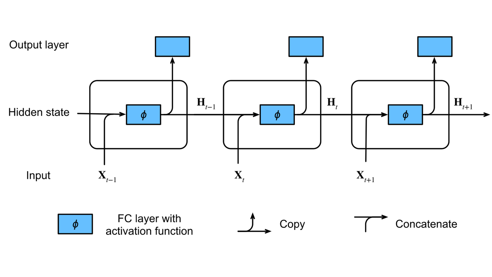
如果任務需要知道事情發生的順序,就要讓前面看到的內容影響後面的計算。RNN 的基本做法,是在讀取每個位置時,把目前輸入和前一步的隱藏狀態一起算進新的狀態。
這篇會追蹤一段三步序列:每一步的數字怎麼來、切成兩段時要傳什麼,以及同一組權重如何從多個時間位置收到梯度。 程式使用手設向量與人工損失,實際做前向、反向與有限差分;沒有把機制檢查包裝成語料訓練、語意理解或預測成效。
隱藏狀態,是下一步會讀取的中間結果
一般逐筆處理的 MLP,可以把目前輸入送進隱藏層,再算輸出。如果每個位置都獨立跑一次,這一步並不會自動知道前一步看過什麼。
RNN 多保留一個狀態。以 column-vector 記號寫一個基本 tanh cell:
a_t = W_ih x_t + b_ih + W_hh h_(t−1) + b_hh
h_t = tanh(a_t)
x_t 是目前輸入,h_(t−1) 是前一步狀態,h_t 是本步更新後的狀態。W_ih 決定輸入怎麼進來,W_hh 決定舊狀態如何參與更新。tanh 逐元素運算,輸出值介於 −1 與 1 之間;有界並不代表它一定記得所有重要資訊。
圖中沿時間排列的三個框,使用的是同一組參數。時間展開表示同一個計算規則被使用三次,不是建立三個彼此獨立的模型。
也要分清「隱藏層」和「隱藏狀態」。前者描述網路內的層;後者是這一步算出、下一步還會用到的值。模型權重和狀態也不同:權重控制更新規則,狀態則隨這條輸入序列變動。
用三個位置,算出順序的影響
本篇設定輸入與狀態都只有兩維,使用三個人工 token 向量:A=[1,0]、B=[0,1]、C=[1,1]。這些數字沒有經過 embedding 訓練,A/B/C 只是讓運算清楚的名稱。
W_ih = [[ 0.4, −0.2],     W_hh = [[ 0.5, 0.15],
        [ 0.1,  0.3]]             [−0.25, 0.4]]

b_ih = [0.05, −0.10]
b_hh = [−0.02, 0.03]
h_0  = [0.10, −0.20]
第一步讀 A,把輸入、舊狀態和兩個偏置相加,得到 a_1=[0.45,−0.075];經過 tanh,變成 h_1≈[0.421899,−0.074860]。第二步不是重新從零開始,而是把這個 h_1 和 B 一起算。
| 時間 | 目前輸入 | 激活前的 a_t | 更新後的 h_t |
|---|---|---|---|
| 1 | A=[1,0] | [0.450000, −0.075000] | [0.421899, −0.074860] |
| 2 | B=[0,1] | [0.029721, 0.094581] | [0.029712, 0.094300] |
| 3 | C=[1,1] | [0.259001, 0.360292] | [0.253361, 0.345471] |
把同一批 token 改成 C、A、B,保持所有權重、偏置及初始狀態不變,最後狀態變成 [0.101611,0.120608]。RNN 在這個例子會區分兩種排列,因為目前輸入遇到的是不同的前一步狀態。
這不保證所有 RNN 都能分辨所有排列。如果參數退化、輸入相同,或重要資訊已在更新中被壓掉,不同序列仍可能得到相同或很接近的狀態。順序會參與計算,不等於模型一定學會了你需要的順序關係。
參數數量不隨序列變長,計算量仍然會增加
本例 PyTorch 單層、單向 RNN 有 12 個純量參數:
| 參數 | 形狀 | 純量數 |
|---|---|---|
| W_ih | 2×2 | 4 |
| W_hh | 2×2 | 4 |
| b_ih | 2 | 2 |
| b_hh | 2 | 2 |
換成 30 步輸入,這四份參數的大小不會因此變成十倍;同一份 W_hh 會被重複使用。但前向要多算時間步,完整反向也要保留及處理更多中間結果,所以不能從參數固定推出時間或記憶體成本固定。
D2L 教材常把有效偏置寫成一個 b_h,並使用 row-batch 公式 X_t W_xh + H_(t−1) W_hh + b_h。PyTorch 儲存 weight_ih 的形狀是 hidden×input,row-batch 寫法要轉置,另外有 bias_ih 與 bias_hh 兩個向量。
本例兩個偏置相加是 [0.03,−0.07]。對照教材時,可以把其中一個設為教材偏置、另一個設零;若兩個都填同一個 b_h,前向就多加了一次。兩個可訓練偏置的有效和能對應單偏置,也不表示同樣學習率下的更新路徑完全一樣。
使用 batch_first=True 時,這個例子的形狀是:
input  : [batch=1, time=3, input_dim=2]
output : [batch=1, time=3, hidden_dim=2]
h_0/h_n: [layers×directions=1, batch=1, hidden_dim=2]
batch_first 改的是 input/output 的排列,不會把 h_n 也改成 batch 在最前面。本例的 output 是每步的隱藏狀態,還不是詞彙機率或退款類別。若要預測,就得另外接適當的輸出頭。
輸出怎麼接,取決於你要預測什麼
同一種狀態更新規則,可以服務不同的任務。序列分類可能把最後狀態交給分類器;逐位置標記則可能每一步都接輸出頭。這不是只換一個函式名字,資料與標籤的對齊也必須改。
| 任務例子 | 輸出在哪裡讀取? | 標籤對應什麼? |
|---|---|---|
| 整句分類 | 例如讀最後有效位置的狀態,再接分類頭 | 整句一個標籤 |
| 逐詞標記 | 每個有效時間位置各接輸出頭 | 每個位置的標籤 |
| 下一字元語言模型 | 每步狀態接詞彙輸出頭 | 後移一個位置的字元 |
這張圖在訓練位置提供來源序列中的真實目前字元,預測後一個字元。生成時,如何把已產生的字元接回去,又是另一個流程;不能從訓練對齊圖直接推出模型已完成自由生成測試。
處理不同長度的文件時,也不能把 padding 當成真正新內容,或直接讀所有樣本共同的最後一格就當作各自的最後有效位置。本篇只跑一條長度為 3、沒有 padding 的序列,沒有驗證變長 batch 或分類頭。
一段文字分兩次讀,要不要保留狀態?
把 A、B、C 切成 [A,B] 與 [C]。第一段讀完後,應把它的最後狀態交給第二段作為起點,才能延續同一段歷史。
本例固定參數、同一條序列、沒有隨機 dropout,實際將兩段輸出串起來,和一次讀完三步的最大差是 0。如果第二段改用零狀態,最後結果是 [0.226028,0.318521],不再等於整段的 [0.253361,0.345471]。
是否延續,取決於資料的身份。連續讀同一本書的相鄰片段,可能需要延續;開始處理另一位客戶的獨立工單,通常就應重設。batch row 順序被 shuffle 後,也不能把前一批某個人的狀態交給下一批另一個人。
PyTorch 不會因為你連續呼叫同一個 nn.RNN,就自動保留前一次狀態。沒有傳 h_0 時,它會建立零初值;想延續必須明確傳入。
重設狀態與 detach 是兩件事。 reset 改了起點數值;detach 保留數值,但不讓後續梯度沿著舊計算圖繼續傳。它不是忘掉前段內容的同義詞。detach 的 tensor 還可能共用底層儲存,若要做原地修改,須另外注意。
本篇分段例子在 no_grad 下檢查前向等價,沒有比較截斷前後的訓練梯度。不能因為 carry 的數字相同,就宣稱截斷 BPTT 的梯度也相同。
BPTT:同一份權重,要接住多次使用的梯度
RNN 的反向傳播仍使用鏈鎖律。把時間步展開後,不只要追蹤前後狀態,也要記得多個位置用的是同一份參數。各次使用產生的梯度必須累加回同一份權重。
本文數值例子使用 tanh,另外設定人工 hidden-state 目標,損失是:
L = 0.5 × Σ_t Σ_k (h_t[k] − target_t[k])²
這是加總,不是預設取平均的 MSE,也不是下一字元交叉熵。三步目標分別是 [0.2,−0.1]、[−0.2,0.3]、[0.1,0.2]。總損失實際為 0.09481626735;它只是為了讓梯度能逐項核算。
在這個 column-vector 記號與損失定義下,可以反向算激活前的梯度:
δ_t = (h_t − target_t + W_hhᵀ δ_(t+1)) ⊙ (1 − h_t²)
∂L/∂W_hh = Σ_t δ_t h_(t−1)ᵀ
⊙ 表示逐元素乘法,最後一步之後的 δ 設零。當前狀態不只影響當前 loss,還會經過後續狀態影響後面的 loss,這就是式子裡有未來梯度那一項的原因。
以 W_hh[0,0] 為例,可以用兩種方式拆開總梯度:
| 拆解位置 | 按權重在該步被使用的貢獻 | 按該步loss對所有早期使用的貢獻 |
|---|---|---|
| 時間1 | 0.032011852 | 0.018240126 |
| 時間2 | 0.113577234 | 0.110452003 |
| 時間3 | 0.004264129 | 0.021161087 |
| 加總 | 0.149853215 | 0.149853215 |
兩欄加總相同,但每一列不是同一件事。左欄的某次參數使用,可能影響後面多個 loss;右欄的某個 loss,可能經過前面多次參數使用。把兩欄逐列畫等號,會誤解共享權重的梯度來源。
完整程式同時比對解析 BPTT、PyTorch autograd 與中央有限差分。有限差分擾動的是 W_hh[0,0],其他值固定,計算 ε=10⁻⁶ 的前後損失差;與反向梯度的誤差約 3.90×10⁻¹³。這支持此例的微分計算,沒有做 optimizer 更新或證明學習成效。
長距離依賴,為什麼仍然難學?
時間越長,早期訊號影響後面狀態的路徑就越長。對 tanh RNN,單步沿狀態傳播的 Jacobian 在 column 記號下包含 diag(1−h_t²) W_hh,完整路徑則包含這些矩陣的連乘。
tanh 接近飽和時,1−h_t² 會很小;多次乘法可能讓早期訊號的梯度逐漸變弱。反過來,某些方向也可能被放大。這不是只看某一個權重大於或小於 1,就能替所有輸入和時間步下定論。
D2L 的線性、無偏置簡化推導用矩陣冪幫助理解這件事,但完整 tanh 網路還受到當下狀態、方向與各步 loss 的影響。不能把一條純線性縮放鏈的指數衰減,直接當成所有 RNN 的實際衰減速度。
截斷 BPTT 在指定邊界停止往更早的計算圖傳梯度,可降低反向計算與儲存負擔,但得到的是截斷後的梯度。它不必把前向狀態歸零,也不代表任何截斷長度都最好。
gradient clipping 則限制當次梯度範數,減少巨大梯度造成的更新問題;它不會替已經消失的訊號補回資訊,也不保證模型學會長期依賴。下一篇的 LSTM/GRU 會改變狀態更新結構,但同樣要理解其條件和限制。
用一支完整程式,核對前向與梯度
下列程式已在 Python 3.10.12、PyTorch 2.3.1+cu118 的既有環境執行,明確使用 CPU/float64。CUDA wheel 名稱不代表本次用了 GPU。程式不下載語料、沒有預訓練模型,也不進行語言模型訓練。
把它存成 rnn_mechanics.py,在已有 PyTorch 的環境執行 python3 rnn_mechanics.py。如果另建 WSL/Linux CPU 環境,可用以下準備方式;本次沒有重新建立或測試這組安裝流程:
python3 -m venv .venv-rnn
source .venv-rnn/bin/activate
python -m pip install torch==2.3.1 --index-url https://download.pytorch.org/whl/cpu
python rnn_mechanics.py
"""CPU/float64 RNN mechanics, with no corpus, fitting or benchmark.

PyTorch stores W_ih/W_hh as (hidden,input)/(hidden,hidden):
h_t = tanh(W_ih x_t + b_ih + W_hh h_prev + b_hh), in column notation.
The plain-Python calculation below uses this orientation explicitly.
"""
import json
import math
import platform
import torch


def plain_recurrence(xs, h0, wi, wh, bi, bh):
    """Independent Python float/math.tanh forward, not a torch rewrite."""
    h = list(h0)
    history, preactivations = [], []
    for x in xs:
        a = [sum(wi[i][j] * x[j] for j in range(2)) + bi[i]
             + sum(wh[i][j] * h[j] for j in range(2)) + bh[i]
             for i in range(2)]
        h = [math.tanh(v) for v in a]
        preactivations.append(a)
        history.append(h)
    return history, preactivations


def main():
    torch.manual_seed(42)  # Initialization is overwritten; not a sampled experiment.
    dtype = torch.float64
    device = torch.device('cpu')
    wi = [[0.4, -0.2], [0.1, 0.3]]
    wh = [[0.5, 0.15], [-0.25, 0.4]]
    bi, bh = [0.05, -0.1], [-0.02, 0.03]
    xs = [[1.0, 0.0], [0.0, 1.0], [1.0, 1.0]]
    initial = [0.1, -0.2]  # Nonzero on purpose: W_hh is active at all three steps.
    targets = [[0.2, -0.1], [-0.2, 0.3], [0.1, 0.2]]
    rnn = torch.nn.RNN(2, 2, num_layers=1, nonlinearity='tanh',
                      bias=True, batch_first=True, dropout=0.0,
                      bidirectional=False, device=device, dtype=dtype)
    with torch.no_grad():
        for name, value in [('weight_ih_l0', wi), ('weight_hh_l0', wh),
                            ('bias_ih_l0', bi), ('bias_hh_l0', bh)]:
            getattr(rnn, name).copy_(torch.tensor(value, dtype=dtype))
    x = torch.tensor([xs], dtype=dtype, device=device)  # batch1,time3,input2
    h0 = torch.tensor([[initial]], dtype=dtype, device=device)  # layer1,batch1,hidden2
    target = torch.tensor([targets], dtype=dtype, device=device)
    python_h, preact = plain_recurrence(xs, initial, wi, wh, bi, bh)
    output, hn = rnn(x, h0)
    manual = torch.tensor([python_h], dtype=dtype)
    torch.testing.assert_close(output, manual, rtol=0, atol=1e-14)
    torch.testing.assert_close(hn[0], output[:, -1], rtol=0, atol=1e-14)

    # Same multiset of tokens, different order, unchanged weights and initial state.
    order = [2, 0, 1]
    with torch.no_grad():
        reordered, reordered_hn = rnn(x[:, order], h0)
        order_difference = (reordered_hn - hn).abs().max().item()
        assert order_difference > 1e-3
        first, state = rnn(x[:, :2], h0)
        second, carried_hn = rnn(x[:, 2:], state)
        carried = torch.cat([first, second], dim=1)
        torch.testing.assert_close(carried, output, rtol=0, atol=1e-14)
        torch.testing.assert_close(carried_hn, hn, rtol=0, atol=1e-14)
        reset_second, reset_hn = rnn(x[:, 2:], torch.zeros_like(state))
        reset_difference = (reset_hn - hn).abs().max().item()
        assert reset_difference > 1e-3

    # Artificial hidden-state squared-error objective, not next-token CE or accuracy.
    # L = 0.5 * sum over all times and both hidden components (h_t - target_t)^2.
    step_losses = 0.5 * (output - target).square().sum(dim=2).squeeze(0)
    per_loss_grad = [torch.autograd.grad(v, rnn.weight_hh_l0, retain_graph=True)[0]
                     for v in step_losses]
    loss = step_losses.sum()
    loss.backward()
    autograd = rnn.weight_hh_l0.grad.detach().clone()
    torch.testing.assert_close(sum(per_loss_grad), autograd, rtol=0, atol=1e-14)

    # Analytic BPTT, pure Python: delta_t = (h_t-y_t + W_hh^T delta_next)
    # * (1-h_t^2). Each use of shared W_hh contributes outer(delta_t,h_prev).
    next_delta = [0.0, 0.0]
    deltas, contributions = [None] * 3, [None] * 3
    for t in range(2, -1, -1):
        delta = [(python_h[t][i] - targets[t][i]
                  + sum(wh[k][i] * next_delta[k] for k in range(2)))
                 * (1 - python_h[t][i] ** 2) for i in range(2)]
        previous = initial if t == 0 else python_h[t-1]
        contributions[t] = [[delta[i] * previous[j] for j in range(2)] for i in range(2)]
        deltas[t], next_delta = delta, delta
    analytic = torch.tensor([[sum(c[i][j] for c in contributions)
                              for j in range(2)] for i in range(2)], dtype=dtype)
    torch.testing.assert_close(analytic, autograd, rtol=0, atol=1e-14)
    assert all(abs(c[0][0]) > 1e-8 for c in contributions)

    # Central finite difference uses the actual torch.nn.RNN forward, not autograd.
    eps = 1e-6
    with torch.no_grad():
        original = rnn.weight_hh_l0[0, 0].item()
        values = []
        for sign in (1, -1):
            rnn.weight_hh_l0[0, 0] = original + sign * eps
            perturbed, _ = rnn(x, h0)
            values.append((0.5 * (perturbed - target).square().sum()).item())
        rnn.weight_hh_l0[0, 0] = original  # Restore the exact original parameter.
    finite_difference = (values[0] - values[1]) / (2 * eps)
    finite_error = abs(finite_difference - autograd[0, 0].item())
    assert finite_error < 1e-8
    assert rnn.weight_hh_l0[0, 0].item() == wh[0][0]

    result = {
        'scope': 'Hand-set CPU mechanics only; no corpus, optimizer, trained task, accuracy or benchmark.',
        'environment': {'python': platform.python_version(), 'torch': torch.__version__,
                        'device': str(output.device), 'dtype': str(output.dtype)},
        'parameters_pytorch_orientation': {'W_ih': wi, 'W_hh': wh, 'b_ih': bi, 'b_hh': bh},
        'inputs': {'token_names': ['A', 'B', 'C'], 'values': xs, 'initial_hidden': initial},
        'shapes': {'input_batch_first': list(x.shape), 'initial_hidden': list(h0.shape),
                   'output_all_hidden': list(output.shape), 'final_hidden': list(hn.shape)},
        'forward': {'preactivations_python': preact, 'hidden_python': python_h,
                    'hidden_torch': output.detach().squeeze(0).tolist(),
                    'max_abs_error': (output - manual).abs().max().item()},
        'order': {'permutation': order, 'token_names': ['C', 'A', 'B'],
                  'reordered_final_hidden': reordered_hn.squeeze().tolist(),
                  'original_final_hidden': hn.detach().squeeze().tolist(),
                  'max_abs_final_difference': order_difference,
                  'interpretation': 'This parameter/input example is order-sensitive; not proof all RNN settings distinguish all permutations.'},
        'chunks': {'split_lengths': [2, 1], 'carry_max_abs_error': (carried-output).abs().max().item(),
                   'reset_to_zero_final_hidden': reset_hn.squeeze().tolist(),
                   'reset_max_abs_final_difference': reset_difference,
                   'interpretation': 'Forward state carry matches full sequence. This no_grad example does not test truncated-BPTT gradients.'},
        'gradient': {'objective': '0.5*sum_t,sum_hidden (h_t-target_t)^2, no averaging',
                     'artificial_targets': targets, 'step_losses': step_losses.detach().tolist(),
                     'loss': loss.item(), 'autograd_shared_W_hh': autograd.tolist(),
                     'analytic_bptt_shared_W_hh': analytic.tolist(),
                     'analytic_deltas_time_order': deltas,
                     'parameter_reuse_contributions_time_order': contributions,
                     'per_time_loss_total_gradients': [g.tolist() for g in per_loss_grad],
                     'partition_warning': 'Reuse contributions include downstream losses; per-time-loss gradients include earlier parameter uses. These are distinct decompositions of the same total.',
                     'finite_difference_W_hh_0_0': finite_difference, 'finite_difference_epsilon': eps,
                     'finite_difference_abs_error': finite_error,
                     'all_three_reuse_contributions_0_0_nonzero': True},
        'checks': 'PASS: Python/nn.RNN forward, all output/h_n shapes, order difference, carry/reset, per-loss sum, analytic BPTT, finite difference.'}
    print(json.dumps(result, ensure_ascii=False, indent=2, allow_nan=False))


if __name__ == '__main__':
    main()
輸出 JSON 中,forward 應列出三步狀態及 Python/PyTorch 的差異;order 列出重排後的末狀態;chunks 比較延續與重設;gradient 則包含兩種分解、解析梯度和有限差分。
這支教學函式固定二維三步,不是任意維度的通用 RNN 函式庫。若修改矩陣、輸入、初始狀態或 loss,數值也會改變;應先重新核算,而不是為了對上本篇輸出調整測試答案。
能逐步追到狀態與梯度,才有辦法判斷問題出在表示、狀態管理、資料對齊,還是優化。把模型換成更複雜的序列網路之前,先讓這些計算邊界清楚,後面的門控、編碼器與注意力才容易理解。
主要來源與版本:
- D2L,Recurrent Neural Networks,狀態更新、共享參數與字元目標對齊;圖片依固定英文版commit轉製。
- D2L,Backpropagation Through Time,計算圖與截斷策略;線性無bias推導的前提和本文tanh例子分開。
- PyTorch 2.3 RNN API,input/output及hidden形狀、兩組偏置與參數定義。
- PyTorch v2.3.1 rnn.py 原碼,本次查核與已安裝檔案逐byte相同;不是沿用新版文件猜測舊版。
- PyTorch 2.3 Tensor.detach,保留數值與停止舊圖梯度的區別。
留言0
登入後就能留言。
登入