往一張照片裡加噪聲,直到幾乎看不見內容,通常不難。真正令人疑惑的是下一段:原圖資訊已經被破壞,模型怎麼還能從噪聲開始,逐步產生一張合理的新影像?
關鍵在於它學習的對象。Diffusion 生成模型不需要知道某個隨機噪聲「原本是哪張照片」,而是透過很多資料與不同噪聲程度的訓練,學習反向走向資料分布的條件轉移。生成時,它從新的噪聲出發;目標是得到符合所學分布的樣本,不是找回某張指定原照。
接續Conditional GAN、Pix2Pix、CycleGAN 與 StyleGAN,本篇聚焦 Ho、Jain、Abbeel 的 2020 年 DDPM。它承接更早的 diffusion probabilistic models,將固定加噪過程、噪聲預測與反向取樣連成可訓練的影像生成方法。這裡先不加入後來的文字引導或 latent diffusion:先把這條基本資料流看清楚,才容易判斷後續方法改了哪一段。
我們會用四組既有原圖讀加噪、係數、網路骨架與分布學習,再以完整 Python 小程式驗三步算術。公式和來源影像不是本站模型訓練結果;小例的已知答案會明確標成 oracle,讓你能區分「數學上可重建」與「模型真的學會預測」兩件事。
先看加噪:固定規則會逐步降低訊號比例
把原始資料記成 x₀,第 t 步的狀態記成 x_t。DDPM 的正向過程是一條固定 Markov chain:下一步只依賴目前狀態與新加入的噪聲。對影像而言,x_t 與原影像維度相同,只是數值逐漸被擾動。
在 DDPM 的變異數保留型參數化中,先指定每一步的 β_t,並定義 α_t=1−β_t。正向式是:
q(x_t | x_(t−1))
  = Normal(mean = sqrt(alpha_t) × x_(t−1), covariance = beta_t × I)

因此可寫成:
x_t = sqrt(alpha_t) × x_(t−1) + sqrt(beta_t) × epsilon_t
其中 epsilon_t 為標準 Gaussian noise,各步獨立。
β_t 是單步加入的噪聲變異數,所以乘在標準噪聲上的振幅是 sqrt(beta_t)。同時,舊狀態也乘上 sqrt(alpha_t)。若只寫成「每一步把原圖加上一點雜訊」,會漏掉這個縮放。
這個過程本身不需要神經網路。選定 schedule 後,訓練程式就知道如何製造各種程度的帶噪輸入。需要學習的是反向:在只看到帶噪狀態時,如何做出接近資料分布的去噪轉移。
還要分清兩種 Gaussian 說法。給定特定 x₀,正向條件分布可以是 Gaussian;把所有不同照片的 x₀ 混合起來,某一步的整體資料分布卻不必是單一 Gaussian。影像中的物體與結構,也不會因為公式出現 Normal 就立即消失。
不必真的加一千次:閉合式直接製造指定程度的帶噪輸入
逐步加噪很適合說明過程,訓練時卻不需要每次從 x₀ 依序算到選中的 t。定義累積乘積:
alpha_bar_t = alpha_1 × alpha_2 × ... × alpha_t

q(x_t | x_0)
  = Normal(sqrt(alpha_bar_t) × x_0, (1 − alpha_bar_t) × I)

x_t = sqrt(alpha_bar_t) × x_0
    + sqrt(1 − alpha_bar_t) × epsilon
其中 epsilon 為一個標準 Gaussian noise。
這給出第 t 步的正確條件邊際分布。如果訓練只需要一個指定噪聲程度的 x_t,可以直接抽 epsilon、代入公式,不必先把前面每一步都跑過。
圖中的藍線逐漸降低,表示原始訊號的係數變小;橘線上升,表示噪聲項的係數變大。兩個係數的平方和是 1,不是兩個係數相加必須為 1。因此它也不是一般圖片編輯器中,兩個透明圖層以加總為 100% 的比例混合。
來源 plot 的橫軸使用從 0 開始的程式索引;論文則以 t=1…T 表示加噪步驟。讀圖時保留這個差別,不把索引 0 誤認為數學上完全沒有加噪的 x₀。原 Ho 論文實驗使用 T=1000、β 從 0.0001 線性增加到 0.02;這張來源保存曲線用於讀係數形狀,不當成本站對某個套件版本的重現驗證。
直接公式也有一個常見陷阱:它保證單一 t 的邊際,不自動保證你另外拼出的整條軌跡具有原 Markov chain 的聯合分布。若每一步的正向噪聲分別為 epsilon₁、epsilon₂,第 2 步其實是:
x_2 = sqrt(alpha_2 × alpha_1) × x_0
    + sqrt(alpha_2 × beta_1) × epsilon_1
    + sqrt(beta_2) × epsilon_2
要拿同一條逐步軌跡對照閉合式,閉合式裡的 epsilon 應是以上噪聲的適當加權合併,而不是直接把 epsilon₂ 原封不動搬進去。當每步噪聲獨立且為標準 Gaussian,合併後重新標準化的噪聲仍是標準 Gaussian;下文用手選常數驗的則是這個代數關係,沒有真的進行 Gaussian 抽樣。
訓練在學什麼:知道加了多少噪聲,拿它當預測目標
現在我們能從真實資料 x₀,直接製造任意 t 的帶噪版本 x_t。訓練時,epsilon 是程式自己抽的,所以答案已知;這提供了不需要人工逐張畫出「正確去噪方向」的監督。
Ho 論文 Algorithm 1 的核心可以分成五個動作:
- 從資料分布抽一個 x₀。
- 均勻抽一個 t,並抽標準 Gaussian epsilon。
- 用閉合式得到 x_t。
- 將 x_t 與 t 交給網路 epsilon_theta,輸出同維度的噪聲預測。
- 依預測噪聲與已知 epsilon 的平方誤差,更新網路參數。
noise_prediction = epsilon_theta(x_t, t)

L_simple = E_(x0,t,epsilon) [||epsilon − epsilon_theta(x_t,t)||^2]
網路需要 t,因為幾乎清楚的影像與幾乎純噪聲的影像,應該採取的轉移不同。它並不是在每一步訓練一個完全獨立的模型;原 DDPM 網路以時間條件接收不同噪聲程度。
這裡預測的是整個 x_t 相對 x₀ 的閉合式噪聲,不是已知原圖上的一張可直接辨識「髒污遮罩」,也不只是最後那次單步加進去的 epsilon_t。不要把「預測噪聲」理解成每個像素都能唯一找回當時抽到的隨機數。
原因是,不同的乾淨資料與噪聲組合,可能產生相同或相近的 x_t。在平方誤差與適當有限矩條件下,理想的最佳函數是給定 x_t、t 的條件平均噪聲;它不必等於每一筆資料背後那次隨機抽樣的真值。訓練可以讓模型掌握資料在不同噪聲尺度下的結構,卻不是把資訊破壞變成一個無歧義的逆函數。Ho 等,§3.2–3.4、Algorithm 1 是這段流程的原始依據。
U-Net 為什麼出現?先把骨架與完整 DDPM 網路分開
帶噪輸入是影像張量,預測目標也是同形狀張量。U 型網路能把較淺的空間資訊,與較深、較大範圍的表徵結合,因此是理解這類預測器的一個入口。
原圖中的小字可以配合這個表讀:
x += h.pop(),不是 U-Net 一定都採用的 concat這張圖的網路在來源前半 toy 中,搭配 uniform noise 混合、直接預測 x₀,也沒有 timestep conditioning。本文只借它解釋 U 型骨架,不把該 toy 的訓練與輸出當成 DDPM epsilon-prediction 實驗。
原 Ho 模型則採另一個 U-Net 設計,包含時間嵌入、GroupNorm 等構件。把 t 轉成 embedding 後提供給預測網路,與單純只接收影像的骨架不是同一回事。輸出是否代表噪聲、原影像或其他參數化,也由訓練目標決定,不能只從 U 型輪廓判定。
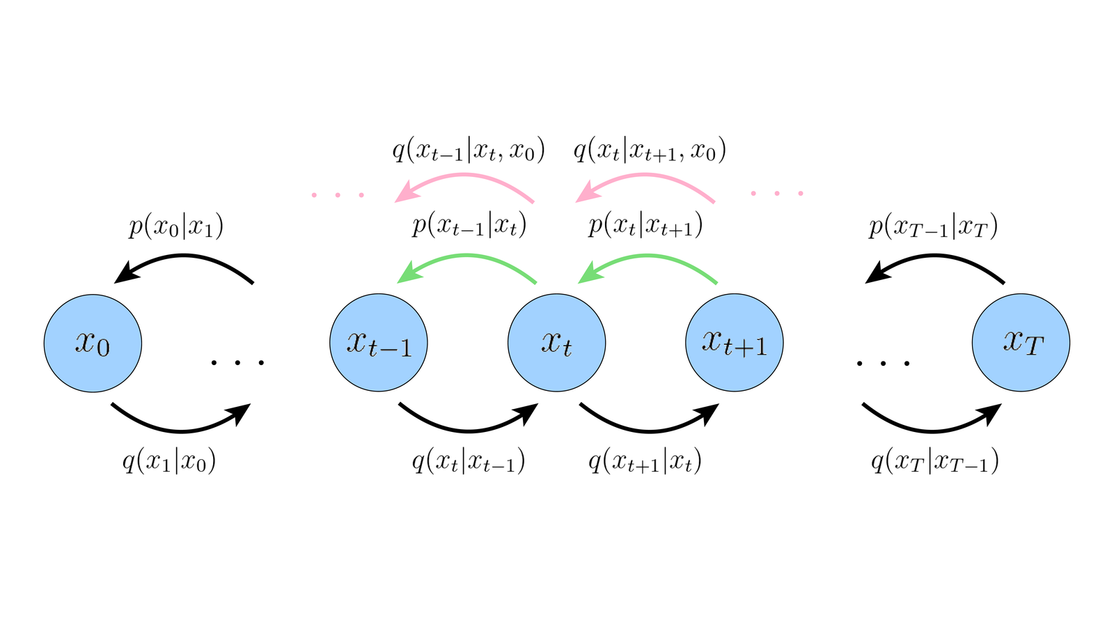
已知原圖的後驗,與生成時可用的反向模型
「既然正向是 Gaussian,反向是不是把公式反過來就好?」這句話必須先問:你反向時,知不知道 x₀?
給定 x₀ 與 x_t,我們可以推得解析的 Gaussian posterior:
q(x_(t−1) | x_t, x_0)
  = Normal(mu_tilde_t, beta_tilde_t × I)

mu_tilde_t = a_t × x_0 + b_t × x_t

a_t = sqrt(alpha_bar_(t−1)) × beta_t / (1−alpha_bar_t)
b_t = sqrt(alpha_t) × (1−alpha_bar_(t−1)) / (1−alpha_bar_t)

beta_tilde_t = beta_t × (1−alpha_bar_(t−1)) / (1−alpha_bar_t)
這是一個很有用的訓練目標,因為訓練資料裡真的有 x₀。但生成時只拿到目前的 x_t,沒有那張正確原圖;一般真正的反向條件 q(x_(t−1)|x_t) 還涉及未知 x₀ 的分布,不能直接冒用上面的已知答案公式。
因此我們學一個模型 p_theta(x_(t−1)|x_t)。在 Ho 的設計中,反向轉移用 Gaussian 參數化,平均值由網路決定,變異數採固定選擇。模型要近似的是適合生成的條件轉移,不是憑空取得每筆資料的 oracle x₀。
為什麼圖裡用分布 matching,而不是說「把每次 x_t 唯一變回前一步」?因為反向通常有不確定性。已知同一個帶噪狀態,仍可能有多個合理的前一步與乾淨資料來源。模型的任務是學會這種條件分布,而不只是為每個輸入指定一個必然正確的歷史。
Noise MSE 與 ELBO 有關,但不是同一個完整式子
原論文先由資料 negative log-likelihood 的變分上界,得到可訓練的分解。對 t>1,有一組 KL 比較已知 x₀ 的 posterior 與 learned reverse;此外還有末端 prior matching,以及 x₁→x₀ 的 decoder 項。
變分上界的結構:
  KL(q(x_T|x_0) || p(x_T))
  + sum_(t=2..T) KL(q(x_(t−1)|x_t,x_0) || p_theta(x_(t−1)|x_t))
  − log p_theta(x_0|x_1)

整體需在相應的資料與正向噪聲分布下取期望。
在固定反向變異數、使用噪聲參數化後,中間項能改寫成帶有時間權重的噪聲平方誤差。Ho 的 L_simple 拿掉這些特定權重,得到前面較簡單的 uniform-t 噪聲預測目標;這個重新加權在來源實驗中帶來較好的取樣品質,但它不是把完整 likelihood bound 原樣抄成一個 MSE。
因此不能說任意一次噪聲平方誤差,就是那張影像 negative log-likelihood 的上界;也不能只比較兩個實作的 MSE 數字,就推論誰的 likelihood 或生成品質一定較好。必須先知道其目標、時間權重與 reduction。
生成流程:從新噪聲開始,每一步只做一個反向轉移
訓練結束後,模型參數固定。Ho Algorithm 2 從標準 Gaussian prior 抽 x_T,接著由 t=T 一直往回走到 1。這些初始噪聲與中途隨機項是新的,不需要對應某張訓練照片的正向噪聲歷史。
噪聲預測可以改寫成反向平均值:
mu_theta(x_t,t)
  = [x_t − beta_t / sqrt(1−alpha_bar_t) × epsilon_theta(x_t,t)]
    / sqrt(alpha_t)

x_(t−1) = mu_theta(x_t,t) + sigma_t × z
在原方法 t>1 的固定變異數選項中,sigma_t² 可以用 β_t,或用上節的 beta_tilde_t。它們都是反向轉移的變異數選擇,不是前面 1−alpha_bar_t 的正向邊際變異數,也不是拿任意標準差直接乘上 z。
在這個 Algorithm 2 裡,t>1 時重新抽標準 Gaussian z;最後 t=1 令 z=0,不再加入這次取樣噪聲,顯示最後的平均預測。這條規則不表示模型已知真 x₀,也不證明它必定還原原照,更不能將所有後續 diffusion sampler 的規則都概括成同一個式子。
你也可以由噪聲預測,先算一個乾淨資料估計:
x0_hat = [x_t − sqrt(1−alpha_bar_t) × epsilon_theta(x_t,t)]
         / sqrt(alpha_bar_t)
但一次 x0_hat 只是根據目前 x_t 的估計,不等於高噪聲輸入已被完全、唯一還原。DDPM 仍依其參數化算下一個反向狀態,再將這個新狀態送進網路。不能把整套生成簡化成「第一步預測噪聲後,一次減乾淨就結束」。
固定 β schedule 與 Gaussian reverse 是本篇原 DDPM 的範圍。它們提供可訓練的近似,不代表有限容量網路、有限資料與任意大 β 都能精確恢復真正反向分布;好看的流程圖本身也不是這種保證。
三步手算:先核閉合式,再看 oracle 到底用了哪些答案
把影像先縮成一個實數,固定 x₀=1.25,手選三個 β 為 [0.1,0.2,0.3],每步噪聲常數為 [-0.5,1.0,-1.5]。這些數字故意方便核算,既不是從 Gaussian 抽出的樣本,也不是原論文的 1000 步 schedule。
| 步 t | alpha_bar_t | 逐步算出的 x_t |
|---|---|---|
| 1 | 0.900 | 1.027740240 |
| 2 | 0.720 | 1.366452411 |
| 3 | 0.504 | 0.321672274 |
第三步雖然數值變小,原始訊號係數仍為 sqrt(0.504),約 0.710,遠不能稱為「只剩純 Gaussian prior」。當次手選噪聲也可能抵消訊號;單看某個值變小,不能證明原圖資訊已經全消失。
在第 2 步,原式可展開成:
x_2 = sqrt(0.72) × 1.25
    + sqrt(0.08) × (−0.5)
    + sqrt(0.20) × 1.0
    ≈ 1.366452411
兩個噪聲係數的平方和為 0.08+0.20=0.28。把這兩個手選噪聲的加權和除以 sqrt(0.28),得到該路徑的有效 epsilon,約 0.577893013;拿它放進閉合式,會得到同一個 x₂。
程式把這個有效值標為 oracle_effective_epsilon,因為它是利用已知的原始值與正向歷史計算出來的答案,不是模型只看 x_t 就預測出的結果。用這個答案重建 x₀,當然能在浮點誤差內回到 1.25;它驗的是代數一致,沒有展示模型學會去噪。
如果把第三步的 oracle epsilon 故意加 0.1,公式重建變成約 1.150796825,誤差為 −0.099203175。由重建公式可以直接得到敏感度:
預測噪聲多了 delta 時:
x0_hat − x0 = −sqrt((1−alpha_bar_t)/alpha_bar_t) × delta
這說明同樣的 epsilon 誤差,會隨時間係數造成不同的重建誤差;不是本篇實測了某個神經網路在不同 t 的能力,也不是新的品質指標。
後驗平均,不必等於手設路徑上的上一個值
在 t=2,用已知 x₀=1.25、x₂≈1.366452411,解析 posterior mean 約為 1.283535870,beta_tilde 為 1/14≈0.071428571。這個平均不同於手設路徑中 x₁≈1.027740240;posterior 描述條件分布,而不是指定那一條歷史必須重新出現。
程式也用另一種二變量 Gaussian conditioning 公式檢查同一個 t=2 mean/variance。t=3 的 posterior variance 則為 21/124≈0.169354839。這些是已知 x₀ 的理論條件值,沒有將它們冒稱為只知道 x_t 時的真實 reverse uncertainty。
再固定一個反向算術用的 z=0.5,可看出變異數選擇如何影響單步:
兩列不是誰比較好的比賽,只是不同固定變異數的算術結果。程式每一列都從儲存的 forward x_t 出發,沒有把這個反向輸出繼續餵給下一列,所以整張表不是一條完成的反向生成軌跡。z=0.5 也是手選常數,不是一次 Gaussian 取樣。
最後 t=1,程式按照 Algorithm 2 把提議的 z=0.5 替為 0。已知 x₀ 的解析 posterior 在這一端退化成 x₀ 本身,variance=0;這個 oracle 條件下的事實,不能用來證明真正 learned model 在最後一步也沒有預測誤差。
完整可重跑程式:用數字檢查哪些等式成立
將下面完整程式存為 diffusion_mechanics.py,以 Python 3 執行。它只使用標準庫,不需安裝 diffusers、PyTorch、模型權重或資料集。保存的實際執行環境是 Python 3.10.12,原型與獨立數值核對均有記錄;這裡沒有宣稱其他平台新環境安裝或 GPU 已驗證。
python3 diffusion_mechanics.py
"""Three-step scalar DDPM arithmetic; no RNG, model, optimizer or image generation."""
import json
import math
import platform


def close(a, b):
    if not math.isclose(a, b, rel_tol=1e-12, abs_tol=1e-12):
        raise AssertionError((a, b))


def main():
    x0 = 1.25
    betas = [0.1, 0.2, 0.3]  # Deliberately large toy schedule, not Ho's trained schedule.
    chosen_eps = [-0.5, 1.0, -1.5]  # Hand-picked constants, NOT Gaussian draws.
    alphas = [1.0 - beta for beta in betas]
    bars = [1.0]
    states = [x0]
    rows = []
    for i, (alpha, beta, eps) in enumerate(zip(alphas, betas, chosen_eps)):
        bars.append(bars[-1] * alpha)
        states.append(math.sqrt(alpha) * states[-1] + math.sqrt(beta) * eps)
        coefficients = [math.sqrt(betas[j] * math.prod(alphas[j + 1:i + 1]))
                        for j in range(i + 1)]
        coeff_sq_sum = sum(c * c for c in coefficients)
        noise_sum = sum(c * e for c, e in zip(coefficients, chosen_eps))
        effective_eps = noise_sum / math.sqrt(1.0 - bars[-1])
        closed = math.sqrt(bars[-1]) * x0 + math.sqrt(1.0 - bars[-1]) * effective_eps
        restored = (states[-1] - math.sqrt(1.0 - bars[-1]) * effective_eps) / math.sqrt(bars[-1])
        close(coeff_sq_sum, 1.0 - bars[-1])
        close(states[-1], closed)
        close(restored, x0)
        delta = 0.1
        perturbed = (states[-1] - math.sqrt(1.0 - bars[-1]) * (effective_eps + delta)) / math.sqrt(bars[-1])
        predicted_error = -math.sqrt((1.0 - bars[-1]) / bars[-1]) * delta
        close(perturbed - x0, predicted_error)
        posterior_var = beta * (1.0 - bars[-2]) / (1.0 - bars[-1])
        x0_coeff = math.sqrt(bars[-2]) * beta / (1.0 - bars[-1])
        xt_coeff = math.sqrt(alpha) * (1.0 - bars[-2]) / (1.0 - bars[-1])
        posterior_mean = x0_coeff * x0 + xt_coeff * states[-1]
        oracle_reverse_mean = (states[-1] - beta * effective_eps / math.sqrt(1.0 - bars[-1])) / math.sqrt(alpha)
        close(posterior_mean, oracle_reverse_mean)
        # Fresh HAND-CHOSEN reverse z, unrelated to the forward epsilon history.
        proposed_z = 0.5
        used_z = proposed_z if i + 1 > 1 else 0.0  # Algorithm 2's last-step rule.
        rows.append({
            't': i + 1, 'alpha': alpha, 'alpha_bar': bars[-1],
            'chosen_step_epsilon': eps, 'sequential_xt': states[-1],
            'forward_noise_coefficients': coefficients,
            'sum_coefficient_squares': coeff_sq_sum, 'forward_marginal_variance': 1.0 - bars[-1],
            'oracle_effective_epsilon': effective_eps, 'closed_form_xt': closed,
            'oracle_reconstructed_x0': restored,
            'epsilon_plus_0_1_reconstruction': perturbed, 'reconstruction_error': predicted_error,
            'posterior_x0_coefficient': x0_coeff, 'posterior_xt_coefficient': xt_coeff,
            'posterior_mean_given_x0': posterior_mean, 'oracle_epsilon_reverse_mean': oracle_reverse_mean,
            'beta_variance': beta, 'posterior_beta_tilde_variance': posterior_var,
            'proposed_hand_chosen_z': proposed_z, 'used_z_after_last_step_rule': used_z,
            'illustrative_step_beta_variance': oracle_reverse_mean + math.sqrt(beta) * used_z,
            'illustrative_step_beta_tilde_variance': oracle_reverse_mean + math.sqrt(posterior_var) * used_z,
        })
    # Independent scalar Gaussian conditioning for t=2 given x0:
    # Cov(x1,x2|x0)=sqrt(alpha2)*Var(x1|x0).
    t = 2
    mean_prev = math.sqrt(bars[t - 1]) * x0
    mean_current = math.sqrt(bars[t]) * x0
    var_prev = 1.0 - bars[t - 1]
    var_current = 1.0 - bars[t]
    cov = math.sqrt(alphas[t - 1]) * var_prev
    conditional_mean = mean_prev + cov / var_current * (states[t] - mean_current)
    conditional_var = var_prev - cov * cov / var_current
    close(conditional_mean, rows[t - 1]['posterior_mean_given_x0'])
    close(conditional_var, rows[t - 1]['posterior_beta_tilde_variance'])
    result = {
        'environment': {'python': platform.python_version(), 'dependencies': 'standard library only', 'numeric_type': 'Python float'},
        'scope': 'Fixed scalar arithmetic. No random sampling, neural network, fitting, image generation or quality evaluation.',
        'x0': x0, 'toy_betas': betas, 'hand_chosen_forward_epsilons': chosen_eps,
        'rows': rows,
        'independent_t2_gaussian_conditioning': {'mean': conditional_mean, 'variance': conditional_var},
        'fixed_epsilon_prediction_squared_error_for_delta_0_1': 0.1 ** 2,
        'limitations': [
            'Effective epsilon is an ORACLE computed from known x0 and the chosen forward history; it is not a learned predictor.',
            'The coefficient-square variance identity has a probabilistic interpretation only with independent standard Gaussian step noises.',
            'Each reverse-step illustration conditions on its stored forward xt; the rows are not a recursively sampled generative trajectory.',
            'The analytic posterior conditions on x0; it is not the generally unavailable true reverse conditional given only xt.',
            'beta and beta_tilde are alternative fixed reverse variance choices for t>1, not the forward marginal variance.',
            'At t=1 sampling adds no z noise. This does not prove a learned model has recovered the original training image.',
            'The final noise squared error is one fixed arithmetic example, not a Monte Carlo estimate or trained objective value.'
        ]
    }
    print(json.dumps(result, ensure_ascii=False, indent=2, allow_nan=False))


if __name__ == '__main__':
    main()
輸出 rows 包含逐步值、係數平方和、閉合式值、oracle 重建、兩種 posterior mean 寫法,以及反向變異數的單步比較。independent_t2_gaussian_conditioning 則是第二種條件化算式的結果。JSON 中相差末幾位的數字是浮點運算差異,檢查用的是數值容差,不要求兩個代數相同式子每一個 bit 都相同。
輸出最後的固定噪聲預測平方誤差約為 0.01,只是固定誤差 0.1 的平方。這支程式沒有抽資料、抽 t 或 Gaussian noise,更沒有更新模型參數;因此這個 0.01 不是 L_simple 的 Monte Carlo 估計,也不是訓練結果。
跑完後,應能回答三件事:閉合式的噪聲為什麼不等於最後一個單步噪聲?解析 posterior 為什麼還要知道 x₀?最後一步不加 z,為什麼仍不保證找回原圖?這三個區分,正是從「會套公式」走向「看懂模型到底學了什麼」的關鍵。
方法、圖片與實作來源
本文以原始方法重新組織教學,另設固定三步算術;沒有重刊 Ho 論文的圖片或將其實驗結果寫成本站成果。原始閱讀範圍以 Ho §2–3.4、Algorithm 1/2、§4 開頭設定,以及 Luo VDM 必要方法 p6末–12 為主,沒有宣稱逐讀兩份論文全部實驗與附錄,也沒有重跑其模型。
- Ho、Jain、Abbeel,Denoising Diffusion Probabilistic Models,NeurIPS 2020:正向閉合式、解析 posterior、epsilon 參數化、L_simple 與取樣演算法。
- Ho 等官方 diffusion_utils.py 固定版本:必要 q_sample/posterior/noise loss/sampling 程式對照,沒有執行 TF1 模型。其程式 t=0 表示數學上的第一步加噪,索引與論文分開讀。
- Calvin Luo,Understanding Diffusion Models: A Unified Perspective,2022,v1:VDM 推導與 Fig. 5 上方純 graph;CC BY 4.0。本篇及封面全部排除該圖下排照片,保留 graph 與 x₀ 條件依賴的省略說明。
- Hugging Face Diffusion Models Course 固定版本 scratch notebook:Jonathan Whitaker 撰寫;取 cell15 自製 BasicUNet 圖與 cell43 原保存曲線。全文 notebook 的 toy 與 DDPM 之比較分開閱讀,本文使用正確的 covariance/噪聲振幅/累積乘積公式,不照搬來源部分文字簡寫。來源程式未在本站執行。
- 該課程固定版本完整 Apache 2.0 LICENSE,以及官方課程重用條款與作者介紹:此為該課程自己的授權,不擴張至其他同名圖片庫或其轉載的第三方論文圖。
- MrAlanKoh 的 Forward Diffusion 作品頁與Axel Tschentscher 的原照片作品頁:圖 1 保留兩位作者與 CC BY-SA 4.0;本次圖片改作維持 SA,其他圖片各依自身授權。
圖像授權副本
以下完整保留圖 2/圖 3 所屬課程的 Apache 2.0 授權副本;這份授權不套到 Commons/Luo 圖片或其他未選取的第三方素材。後面的 notice 是本次選圖署名與變更紀錄,不是宣稱課程原本附有同名 NOTICE。
                                 Apache License
                           Version 2.0, January 2004
                        http://www.apache.org/licenses/

   TERMS AND CONDITIONS FOR USE, REPRODUCTION, AND DISTRIBUTION

   1. Definitions.

      "License" shall mean the terms and conditions for use, reproduction,
      and distribution as defined by Sections 1 through 9 of this document.

      "Licensor" shall mean the copyright owner or entity authorized by
      the copyright owner that is granting the License.

      "Legal Entity" shall mean the union of the acting entity and all
      other entities that control, are controlled by, or are under common
      control with that entity. For the purposes of this definition,
      "control" means (i) the power, direct or indirect, to cause the
      direction or management of such entity, whether by contract or
      otherwise, or (ii) ownership of fifty percent (50%) or more of the
      outstanding shares, or (iii) beneficial ownership of such entity.

      "You" (or "Your") shall mean an individual or Legal Entity
      exercising permissions granted by this License.

      "Source" form shall mean the preferred form for making modifications,
      including but not limited to software source code, documentation
      source, and configuration files.

      "Object" form shall mean any form resulting from mechanical
      transformation or translation of a Source form, including but
      not limited to compiled object code, generated documentation,
      and conversions to other media types.

      "Work" shall mean the work of authorship, whether in Source or
      Object form, made available under the License, as indicated by a
      copyright notice that is included in or attached to the work
      (an example is provided in the Appendix below).

      "Derivative Works" shall mean any work, whether in Source or Object
      form, that is based on (or derived from) the Work and for which the
      editorial revisions, annotations, elaborations, or other modifications
      represent, as a whole, an original work of authorship. For the purposes
      of this License, Derivative Works shall not include works that remain
      separable from, or merely link (or bind by name) to the interfaces of,
      the Work and Derivative Works thereof.

      "Contribution" shall mean any work of authorship, including
      the original version of the Work and any modifications or additions
      to that Work or Derivative Works thereof, that is intentionally
      submitted to Licensor for inclusion in the Work by the copyright owner
      or by an individual or Legal Entity authorized to submit on behalf of
      the copyright owner. For the purposes of this definition, "submitted"
      means any form of electronic, verbal, or written communication sent
      to the Licensor or its representatives, including but not limited to
      communication on electronic mailing lists, source code control systems,
      and issue tracking systems that are managed by, or on behalf of, the
      Licensor for the purpose of discussing and improving the Work, but
      excluding communication that is conspicuously marked or otherwise
      designated in writing by the copyright owner as "Not a Contribution."

      "Contributor" shall mean Licensor and any individual or Legal Entity
      on behalf of whom a Contribution has been received by Licensor and
      subsequently incorporated within the Work.

   2. Grant of Copyright License. Subject to the terms and conditions of
      this License, each Contributor hereby grants to You a perpetual,
      worldwide, non-exclusive, no-charge, royalty-free, irrevocable
      copyright license to reproduce, prepare Derivative Works of,
      publicly display, publicly perform, sublicense, and distribute the
      Work and such Derivative Works in Source or Object form.

   3. Grant of Patent License. Subject to the terms and conditions of
      this License, each Contributor hereby grants to You a perpetual,
      worldwide, non-exclusive, no-charge, royalty-free, irrevocable
      (except as stated in this section) patent license to make, have made,
      use, offer to sell, sell, import, and otherwise transfer the Work,
      where such license applies only to those patent claims licensable
      by such Contributor that are necessarily infringed by their
      Contribution(s) alone or by combination of their Contribution(s)
      with the Work to which such Contribution(s) was submitted. If You
      institute patent litigation against any entity (including a
      cross-claim or counterclaim in a lawsuit) alleging that the Work
      or a Contribution incorporated within the Work constitutes direct
      or contributory patent infringement, then any patent licenses
      granted to You under this License for that Work shall terminate
      as of the date such litigation is filed.

   4. Redistribution. You may reproduce and distribute copies of the
      Work or Derivative Works thereof in any medium, with or without
      modifications, and in Source or Object form, provided that You
      meet the following conditions:

      (a) You must give any other recipients of the Work or
          Derivative Works a copy of this License; and

      (b) You must cause any modified files to carry prominent notices
          stating that You changed the files; and

      (c) You must retain, in the Source form of any Derivative Works
          that You distribute, all copyright, patent, trademark, and
          attribution notices from the Source form of the Work,
          excluding those notices that do not pertain to any part of
          the Derivative Works; and

      (d) If the Work includes a "NOTICE" text file as part of its
          distribution, then any Derivative Works that You distribute must
          include a readable copy of the attribution notices contained
          within such NOTICE file, excluding those notices that do not
          pertain to any part of the Derivative Works, in at least one
          of the following places: within a NOTICE text file distributed
          as part of the Derivative Works; within the Source form or
          documentation, if provided along with the Derivative Works; or,
          within a display generated by the Derivative Works, if and
          wherever such third-party notices normally appear. The contents
          of the NOTICE file are for informational purposes only and
          do not modify the License. You may add Your own attribution
          notices within Derivative Works that You distribute, alongside
          or as an addendum to the NOTICE text from the Work, provided
          that such additional attribution notices cannot be construed
          as modifying the License.

      You may add Your own copyright statement to Your modifications and
      may provide additional or different license terms and conditions
      for use, reproduction, or distribution of Your modifications, or
      for any such Derivative Works as a whole, provided Your use,
      reproduction, and distribution of the Work otherwise complies with
      the conditions stated in this License.

   5. Submission of Contributions. Unless You explicitly state otherwise,
      any Contribution intentionally submitted for inclusion in the Work
      by You to the Licensor shall be under the terms and conditions of
      this License, without any additional terms or conditions.
      Notwithstanding the above, nothing herein shall supersede or modify
      the terms of any separate license agreement you may have executed
      with Licensor regarding such Contributions.

   6. Trademarks. This License does not grant permission to use the trade
      names, trademarks, service marks, or product names of the Licensor,
      except as required for reasonable and customary use in describing the
      origin of the Work and reproducing the content of the NOTICE file.

   7. Disclaimer of Warranty. Unless required by applicable law or
      agreed to in writing, Licensor provides the Work (and each
      Contributor provides its Contributions) on an "AS IS" BASIS,
      WITHOUT WARRANTIES OR CONDITIONS OF ANY KIND, either express or
      implied, including, without limitation, any warranties or conditions
      of TITLE, NON-INFRINGEMENT, MERCHANTABILITY, or FITNESS FOR A
      PARTICULAR PURPOSE. You are solely responsible for determining the
      appropriateness of using or redistributing the Work and assume any
      risks associated with Your exercise of permissions under this License.

   8. Limitation of Liability. In no event and under no legal theory,
      whether in tort (including negligence), contract, or otherwise,
      unless required by applicable law (such as deliberate and grossly
      negligent acts) or agreed to in writing, shall any Contributor be
      liable to You for damages, including any direct, indirect, special,
      incidental, or consequential damages of any character arising as a
      result of this License or out of the use or inability to use the
      Work (including but not limited to damages for loss of goodwill,
      work stoppage, computer failure or malfunction, or any and all
      other commercial damages or losses), even if such Contributor
      has been advised of the possibility of such damages.

   9. Accepting Warranty or Additional Liability. While redistributing
      the Work or Derivative Works thereof, You may choose to offer,
      and charge a fee for, acceptance of support, warranty, indemnity,
      or other liability obligations and/or rights consistent with this
      License. However, in accepting such obligations, You may act only
      on Your own behalf and on Your sole responsibility, not on behalf
      of any other Contributor, and only if You agree to indemnify,
      defend, and hold each Contributor harmless for any liability
      incurred by, or claims asserted against, such Contributor by reason
      of your accepting any such warranty or additional liability.

   END OF TERMS AND CONDITIONS

   APPENDIX: How to apply the Apache License to your work.

      To apply the Apache License to your work, attach the following
      boilerplate notice, with the fields enclosed by brackets "[]"
      replaced with your own identifying information. (Don't include
      the brackets!)  The text should be enclosed in the appropriate
      comment syntax for the file format. We also recommend that a
      file or class name and description of purpose be included on the
      same "printed page" as the copyright notice for easier
      identification within third-party archives.

   Copyright [yyyy] [name of copyright owner]

   Licensed under the Apache License, Version 2.0 (the "License");
   you may not use this file except in compliance with the License.
   You may obtain a copy of the License at

       http://www.apache.org/licenses/LICENSE-2.0

   Unless required by applicable law or agreed to in writing, software
   distributed under the License is distributed on an "AS IS" BASIS,
   WITHOUT WARRANTIES OR CONDITIONS OF ANY KIND, either express or implied.
   See the License for the specific language governing permissions and
   limitations under the License.
Hugging Face Diffusion Models Course
Source: https://github.com/huggingface/diffusion-models-class/tree/72bf3dd739da641075dcff0ee54ce28e7a38a8ab
Diffusion Models from Scratch notebook written by Jonathan Whitaker for the Hugging Face course. Course authors: Jonathan Whitaker and Lewis Tunstall.
Selected images: original embedded BasicUNet diagram (cell 15); original saved noise-schedule output (cell 43).
Licensed under the Apache License, Version 2.0. Full license accompanies these images.
Changes: proportional resizing and white background/layout. The mobile BasicUNet image shows the whole diagram first, followed by four original legend-box crops enlarged vertically; these repeat source pixels and add no layers or paths. No labels, curves, arrows or data redrawn.
The course repository contains no standalone NOTICE file at this pinned commit. This file records attribution for this selection, not an assertion that it was an upstream NOTICE.
留言0
登入後就能留言。
登入