
把每日銷量交給 LSTM,不會自動比「照上週同一天」更好。模型能讀取順序,只代表它多了一種處理歷史的方式;這個方式是否值得,要看我們需要的資訊、手上的資料,以及真正交付的預測任務。
有用的比較,會讓候選站在相同時間點:能看到哪些歷史?一次要預測幾天?後續會拿到真值,還是必須接回自己的預測?然後才看它換來多少增益。
上一篇用 lag 與 rolling 把序列變成表格。這篇改把最近十四個觀測直接交給兩個小網路:一個 MLP、一個 LSTM。它們接受相同輸入、同樣一次預測未來十四天,再和季節基線比較。這是實際訓練的 CPU 教學案例,資料仍是人工設計,沒有拿它當成真實產業或架構排名。
先對齊任務,才比較模型名稱
假設目前要替單一門市一次準備未來十四天的需求預測。第一天之後,真實需求尚未到達,所以不論用 MLP 或 LSTM,都不能在後段偷看測試區間的昨日真值。
公平比較至少要先對齊三件事:可用資訊、要預測的範圍、選模型的時間。模型可以有不同的參數與假設,但如果其中一個能看到更多歷史、額外日曆或未來天氣,差異就不全是架構造成。
季節基線只使用最後七點,作用是提供一個容易核算的季節參照;兩個神經網路才是使用相同十四筆歷史的架構比較。這也與上一篇森林的特徵契約不同:森林拿到 lag1、lag7、rolling7 和日曆指示,不能跨篇把分數拼成「森林、MLP、LSTM 誰最好」的公平排行榜。
十四筆歷史,可以攤平成向量,也可以依序讀
把最近十四筆按時間排好,MLP 可以把它們當成十四個有固定位置的欄位。第一欄是較早的觀測,最後一欄是最新值。攤平不等於把順序打亂:欄位位置仍保留了先後,只是模型沒有循環狀態或跨時間共用的轉移規則。
LSTM 則依次讀入這十四個值。讀到下一個時間點時,用前一步的 hidden/cell state 和目前輸入更新狀態,最後再用最新 hidden state 產生下一點預測。
這兩種方式有不同的結構偏好。MLP 對固定位置使用自己的連結權重;LSTM 在同一個 window 的各時間步重複使用同一組 cell 參數。後者能把「讀入一筆後怎麼更新狀態」學成共享規則,但共享規則不保證對每個資料生成機制都有優勢。
尤其要問清楚狀態保留多久。本文每個 window 都從零 hidden/cell state 開始,沒有把上一個訓練樣本的狀態接到下一個樣本。因此它只能透過這十四個輸入更新當次狀態,沒有跨 window 記住任意長歷史。換成 LSTM 名稱,不會讓沒提供的第十五天以前的觀測自動出現。
LSTM 的門控制狀態,但不替我們判定預測是否成功
LSTM 的 input、forget、output gate 是連續的控制值,不是預先寫好的「遇到週末就記住」規則。它們與候選內容一起,決定 cell state 要保留什麼、加入什麼,以及 hidden state 如何輸出。
c(t) = f(t) * c(t-1) + i(t) * g(t)
h(t) = o(t) * tanh(c(t))

f、i、o:sigmoid gates,逐元素控制
 g:tanh candidate,提出要寫入的內容
 c:cell state
 h:hidden state
這條狀態更新路徑讓 LSTM 能調整訊息保留方式,但不保證所有長序列梯度都維持不變,也不保證它一定找到對需求預測有用的訊號。若要細看各門、兩種 bias 與 GRU 的差異,可以接著讀 LSTM 與 GRU 的機制篇;本篇把重點放在預測資料流與比較條件。
本文 LSTM 的 input_size=1、hidden_size=8,最後接一個 8→1 線性 head。PyTorch 這個設定有兩組 gate bias,因此參數量要把兩組都算進去:
LSTM cell:
  輸入權重 4*8*1 = 32
  hidden 權重 4*8*8 = 256
  兩組 bias 2*(4*8) = 64
  cell 合計 352
線性 head:8*1 + 1 = 9
總計:361

MLP:14 → 16 → 1,中間 Tanh
  14*16 + 16 + 16*1 + 1 = 257
兩者的參數量不同,所以相同訓練步數不代表相同容量,也不代表已給每個架構最適合的訓練預算。本例是在固定設定下觀察,沒有宣稱完成公平的最佳化調參競賽。
建立滑動視窗時,先把 target 與 batch 維度分開
對第 t 點的訓練列,我們取 t−14 到 t−1 共十四筆作輸入,答案是 y(t)。以零起算,第一個可用 target 是 index 14,之前歷史不足的 target 不補成假資料。
單一樣本:過去14點 → 下一點
訓練 x:batch × 14 × 1
訓練 y:batch

LSTM output:batch × 14 × 8
LSTM h_n/c_n:1 × batch × 8
線性 head:取最後時間步的8維hidden → 1個預測
batch_first=True 改變 input/output 的 batch 位置,不會把 h_n/c_n 也改成 batch 在第一維。這個模型只有一層、單向、沒有 projection,所以 state 的第一維是 1;也不能把 cell state 當成最後的標量預測。
例如起點 126 只拿到 index 0–125,扣掉十四個起始點,訓練 x 是 112×14×1。樣本之間的 window 有重疊,這不會讓每列變成獨立資料集;訓練 fit、驗證評分與不確定性推論都要記得這點。
接著做正規化。每個起點各自用當時的訓練 prefix 算平均與 population standard deviation,再用同一組數字轉換該次模型的輸入和 target:
z(t) = [y(t) - train_mean] / train_population_std
反轉:ŷ(t) = ẑ(t) * train_population_std + train_mean
不能先用全部 168 點算出平均與標準差,再假裝站在 index 125 預測未來。程式的 scale 只來自當時的訓練資料,後續十四步的預測也沿用它;不是每走一步就偷用新真值重算。
一步曲線貼近,不等於一次預測很遠也會貼近
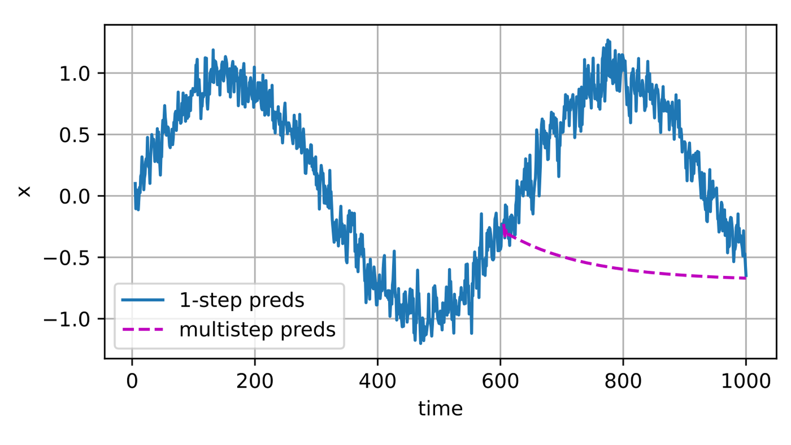
先看一個有助於辨別任務的來源例子。D2L 用正弦加雜訊生成序列,再用前四個觀測訓練線性回歸。這幾張圖都不是本文的 LSTM 結果。
來源把前 600 個訓練樣本交給線性回歸:每個樣本看四個歷史,按一開始的時間記號,訓練 target 是 x5 到 x604。它可以用實際觀察的四筆歷史,對各時間點做一步預測。
當我們改問「只知道 x604,要一路預測到 x1000」,後續輸入就不再是原本的實際觀察,而必須包含自己的預測。模型沒有重新變成另一種神經網路,變的是它能取得的資訊。
圖中的差異提醒我們,時間序列驗證不能只列出「有沒有 holdout」。還要交代每一步的特徵來自真實觀察還是先前預測。遞迴可能把偏差繼續帶進輸入,但每個模型、資料與 horizon 的實際影響都要評估;這個線性來源例子不能證明 LSTM 都會失敗,或每多一步誤差一定上升。
本文兩個網路都做相同的十四步遞迴。第一步讀最後十四個 normalized 真值,輸出一個 normalized 預測,把它接回 prefix;第二步開始,window 就逐步混入自己的預測。直到最後都不拿段內真值更新。
實作:兩個網路、三個種子、相同十四天任務
人工資料共 168 點,包含每步 0.1 的成長、七點週期形狀與五點確定擾動。這些規律是作者設計,不是從外部真實需求資料抽樣。選擇週期、網路寬度、訓練步數與種子也都事先固定。
| 用途 | 可見 prefix | 神經網路訓練 target | 一次預測 |
|---|---|---|---|
| 驗證一 | 0–125 | 14–125 | 126–139 |
| 驗證二 | 0–139 | 14–139 | 140–153 |
| 最後評估 | 0–153 | 14–153 | 154–167 |
每個神經網路各用 seed 7、19、41 訓練。對每次 fit,以全部訓練 window 計算 MSE,做 200 次 full-batch Adam 更新,lr=.01。每次更新前清梯度,再 backward/step;不是只做 200 次 forward,也不是用手填的權重輸出結果。
程式中變數叫 EPOCHS,這裡每輪只有一次 full-batch 更新,因此實際就是 200 次更新。這個關係不能直接套到有很多 mini-batch 的其他訓練流程。也沒有早停、調參搜尋或訓練時間 benchmark。
下面是實際執行環境。wheel 名稱含 cu118,但此程式指定的運算是 CPU float64,沒有測 GPU。
Python 3.10.12
torch 2.3.1+cu118
CPU / float64 / single thread
將完整程式存成檔案,在已安裝對應 PyTorch 的環境執行:
python3 lstm_and_mlp_forecasts.py > stdout.json
requirements 可記為以下版本;本文驗證的是上述已存在的環境,沒有宣稱全新 pip 安裝、其他 wheel 或不同平台都已逐 byte 重現。
torch==2.3.1
"""Actual CPU LSTM/MLP fits on an original deterministic teaching sequence.

All models forecast the same 14 future points from the same observed prefix.
Neural networks see 14 lag values; both reset state for every input window.
"""
import json
import platform

import torch
from torch import nn


WINDOW = 14
HORIZON = 14
EPOCHS = 200
SEEDS = (7, 19, 41)
MODELS = ("seasonal_naive", "mlp", "lstm")
PATTERN = (-6, -3, 0, 2, 5, 11, 8)
DISTURBANCE = (-1, 0, 1, 0, -1)
SERIES = [50 + 0.1 * t + PATTERN[t % 7] + DISTURBANCE[t % 5]
          for t in range(168)]


class ForecastNet(nn.Module):
    def __init__(self, kind):
        super().__init__()
        self.kind = kind
        if kind == "lstm":
            self.recurrent = nn.LSTM(1, 8, batch_first=True)
            self.head = nn.Linear(8, 1)
        else:
            assert kind == "mlp"
            self.mlp = nn.Sequential(nn.Flatten(), nn.Linear(WINDOW, 16),
                                     nn.Tanh(), nn.Linear(16, 1))

    def forward(self, inputs):
        if self.kind == "mlp":
            return self.mlp(inputs).squeeze(-1)
        # No h0/c0 supplied: each window starts from zeros, no state carryover.
        outputs, _ = self.recurrent(inputs)
        return self.head(outputs[:, -1, :]).squeeze(-1)


def neural_forecast(history, kind, seed):
    torch.manual_seed(seed)
    raw = torch.tensor(history, dtype=torch.float64)
    center = raw.mean()
    scale = raw.std(correction=0)
    assert scale > 0
    normalized = (raw - center) / scale
    x = torch.stack([normalized[t-WINDOW:t] for t in range(WINDOW, len(raw))])
    x = x.unsqueeze(-1)
    y = normalized[WINDOW:]
    assert x.shape == (len(history) - WINDOW, WINDOW, 1)
    net = ForecastNet(kind).double()
    optimizer = torch.optim.Adam(net.parameters(), lr=0.01)
    net.train()
    initial_loss = float(nn.functional.mse_loss(net(x), y).detach())
    for _ in range(EPOCHS):
        optimizer.zero_grad()
        loss = nn.functional.mse_loss(net(x), y)
        loss.backward()
        optimizer.step()
    net.eval()
    with torch.no_grad():
        final_loss = float(nn.functional.mse_loss(net(x), y))
        prefix = normalized.tolist()
        forecast = []
        for _ in range(HORIZON):
            window = torch.tensor(prefix[-WINDOW:], dtype=torch.float64).reshape(1, WINDOW, 1)
            value = float(net(window)[0])
            prefix.append(value)
            forecast.append(value * float(scale) + float(center))
    assert torch.isfinite(torch.tensor(forecast)).all()
    return forecast, {"seed": seed, "training_target_indices": [WINDOW, len(history)-1],
        "input_shape": list(x.shape), "train_only_mean": float(center),
        "train_only_population_std": float(scale),
        "parameter_count": sum(p.numel() for p in net.parameters()),
        "initial_scaled_training_MSE": initial_loss, "final_scaled_training_MSE": final_loss}


def mae(truth, prediction):
    return sum(abs(a-b) for a, b in zip(truth, prediction)) / len(truth)


def evaluate(origin):
    history = SERIES[:origin]
    truth = SERIES[origin:origin + HORIZON]
    rows = []
    for kind in MODELS:
        seeds = (None,) if kind == "seasonal_naive" else SEEDS
        for seed in seeds:
            if seed is None:
                predicted = [history[-7 + h % 7] for h in range(HORIZON)]
                metadata = {"seed": None, "parameter_count": 0}
            else:
                predicted, metadata = neural_forecast(history, kind, seed)
            rows.append({"origin": origin, "forecast_indices": [origin, origin+HORIZON-1],
                "model": kind, **metadata, "prediction": [round(v, 8) for v in predicted],
                "truth": [round(v, 8) for v in truth], "MAE": mae(truth, predicted)})
    return rows


def main():
    torch.set_num_threads(1)
    torch.use_deterministic_algorithms(True)
    validation = evaluate(126) + evaluate(140)
    scores = {kind: sum(r["MAE"] for r in validation if r["model"] == kind)
              / sum(r["model"] == kind for r in validation) for kind in MODELS}
    selected = min(MODELS, key=lambda kind: (scores[kind], MODELS.index(kind)))
    # Freeze model-family selection before examining final-block errors.
    final = evaluate(154)
    final_scores = {kind: sum(r["MAE"] for r in final if r["model"] == kind)
                    / sum(r["model"] == kind for r in final) for kind in MODELS}
    print(json.dumps({"scope": "Hand-set 168-point daily signal, actual CPU float64 training. "
        "Fixed architectures/200 updates/three initialization seeds, no external benchmark.",
        "versions": {"python": platform.python_version(), "torch": torch.__version__},
        "device": "cpu", "dtype": "float64", "threads": torch.get_num_threads(),
        "window": WINDOW, "horizon": HORIZON, "epochs": EPOCHS, "seeds": SEEDS,
        "series": [round(v, 8) for v in SERIES], "validation": validation,
        "mean_validation_MAE_across_origins_and_seeds": scores,
        "selected_before_final_evaluation": selected, "final": final,
        "final_mean_individual_seed_MAE": final_scores,
        "limits": ["The mean of individual seed MAEs is not an ensemble forecast MAE.",
            "Three initialization seeds are not independent datasets or a significance test.",
            "Training histories overlap; 14-day blocks never receive intermediate actuals.",
            "Scalers use training-prefix observations only; no final-block scaling statistics.",
            "Only 200 fixed updates, not proof of optimizer convergence or fair tuning budgets.",
            "LSTM and MLP have different parameter counts but identical observed lag inputs.",
            "State resets for each window; no claim of learning beyond the 14-value context.",
            "Same-environment deterministic settings do not promise cross-platform byte identity.",
            "No empirical real-data performance, calibrated intervals, or general architecture ranking."]},
        ensure_ascii=False, indent=2))


if __name__ == "__main__":
    main()
實際 JSON 的驗證摘要如下。兩個起點、各三種子的神經網路 MAE 共六個值取平均;基線在兩個起點各算一次。
{
  "mean_validation_MAE_across_origins_and_seeds": {
    "seasonal_naive": 1.514285714285713,
    "mlp": 0.4754750894753413,
    "lstm": 1.3062758667841428
  },
  "selected_before_final_evaluation": "mlp"
}
| 固定候選 | 驗證平均 MAE | 最後區段 MAE |
|---|---|---|
| 季節 naive | 1.514286 | 1.292857 |
| MLP,individual-seed MAE 平均 | 0.475475 | 0.461417 |
| LSTM,individual-seed MAE 平均 | 1.306276 | 1.394659 |
這裡先由驗證選 MLP,再計算最後區段,最後也仍是 MLP 較好。LSTM 的最後平均甚至比季節基線差。這些結果應該照實呈現,卻不能推成「LSTM 家族不適合時間序列」:我們只比較一條人工訊號、兩個小架構與固定訓練設定。
看懂 loss、種子與預測分數各自代表什麼
先看一個單次 fit:起點 126、seed 7 的 MLP,scaled training MSE 從約 0.865644 降到 0.000598;LSTM 從約 1.026295 降到 0.222446。這證明在這兩次訓練裡 loss 有下降,不代表已達到最佳解,也不能把 normalized MSE 直接和原始尺度上的 MAE 比數字大小。
再看最後區段的逐種子結果,才不會讓平均數隱藏差異:
| seed | MLP 最後 MAE | LSTM 最後 MAE |
|---|---|---|
| 7 | 0.392685 | 1.407778 |
| 19 | 0.473781 | 1.916603 |
| 41 | 0.517785 | 0.859596 |
同一個 LSTM 設定,在這三個初始化下有差異;但三種 seed 仍是在同一條資料上訓練,不是三個獨立資料集,也不是顯著性檢定。不能在看過最後結果後,只挑 seed 41 當成一開始選定的模型成績。
本例報告的還是「每個模型先算 MAE,再把三個 MAE 平均」,沒有先把三條預測平均成 ensemble。兩種算法並不相同:誤差在預測平均時可能互相抵銷。若日後要部署集成,應把它當作一個明確的候選,在驗證階段評估其預測、成本與規則。
相同 200 次更新也不是公平調參的全部。架構可能需要不同 learning rate、正則化、window 長度或訓練次數。這裡把它們固定,是為了讓程式短且可核對;若要為真實專案作選型,還需要把預算與搜尋方式設計成可比較的實驗。
什麼情況下,值得把 LSTM 加進候選?
先把「值得嘗試」和「已證明值得部署」分開。若資料裡真的有需要依序整合的訊息,並且有足夠的歷史或可合理共享的多序列資料,LSTM 可以是候選;它是否帶來收益,仍要回到保留時間順序的驗證與實際維護成本。
本例沒有量測 latency、訓練時間或真實業務收益,因此不能由 361 個參數就斷言 LSTM 在產品上很便宜,也不能由某一次 CPU 實跑推論所有部署環境。
對這一題最實用的判準,是在同樣能取得的資訊與同樣要交付的 horizon 下,深度模型是否持續改善你真正關心的誤差,改善是否足以負擔訓練與維護。若答案還不清楚,可先回到可用資訊、horizon 與驗證切分,讓後續的增益有可檢查的依據。
來源與圖像授權
本文新增的是固定人工訊號上的完整 CPU 訓練、兩個驗證起點的選模、三個初始化種子的逐次結果,以及相同十四點輸入與遞迴契約的拆解。來源中的線性回歸曲線沒有被改稱本站 LSTM 成果。
- D2L 四位作者 Aston Zhang、Zachary C. Lipton、Mu Li、Alexander J. Smola:Working with Sequences 原章、預測段與原圖、LSTM 原章、固定版本章節 Markdown、固定 README 授權說明、CC BY-SA 4.0。序列章的圖來自官方 1.0.3 頁面保存的 SVG,gate 圖另依 LSTM 原章對應圖。來源檔案以雜湊保存,不冒稱所有輸出 SVG 都是該 repo commit 內的檔案。書籍圖像與本文圖像改作依 CC BY-SA 4.0,圖說保留具體來源與變更;不拿 sample-code MIT 當成圖片授權。
- PyTorch:2.3 LSTM API、2.3 Reproducibility。程式以實際安裝的 2.3.1 docstring/source 與 CPU 執行核對;文件網址和 wheel 執行紀錄分開。相同 seed 與 deterministic 設定不保證跨版本、裝置或平台逐 byte 一致。
以下保留選用圖的完整署名、來源、改作與相同授權聲明。
Source image credits and license

Four sequence source figures and one selected LSTM gate figure are from Dive into Deep Learning, English edition, by Aston Zhang, Zachary C. Lipton, Mu Li, and Alexander J. Smola. The book visuals are licensed under Creative Commons Attribution-ShareAlike 4.0 International (CC BY-SA 4.0): https://creativecommons.org/licenses/by-sa/4.0/ . The sample-code license is separate and is not relied upon for these figures.

The four sequence SVGs were obtained from the live D2L 1.0.3 chapter image URLs and locally hash-pinned. Repository revision 23d7a5aecceee57d1292c56e90cce307f183bb0a identifies the chapter Markdown, README and license; these rendered output SVGs are not claimed to be files in that commit. The selected LSTM gate image is rendered from the pinned D2L LSTM source SVG.

Changes: the original source SVGs are rendered on white at 1400px width; two forecast mobile derivatives show the complete chart first, followed by enlarged original plot-interior and complete-legend crops; the cover fits the complete one-step-vs-recursive plot proportionally to a white 1600x900 canvas. No data, labels, lines, arrows or chart elements were added or redrawn. Shared adaptations are offered under CC BY-SA 4.0. No additional restrictions are applied to recipients exercising the license rights.

The D2L sequence forecast example is synthetic noisy-sine data fitted with linear regression, not an LSTM result.
留言0
登入後就能留言。
登入