
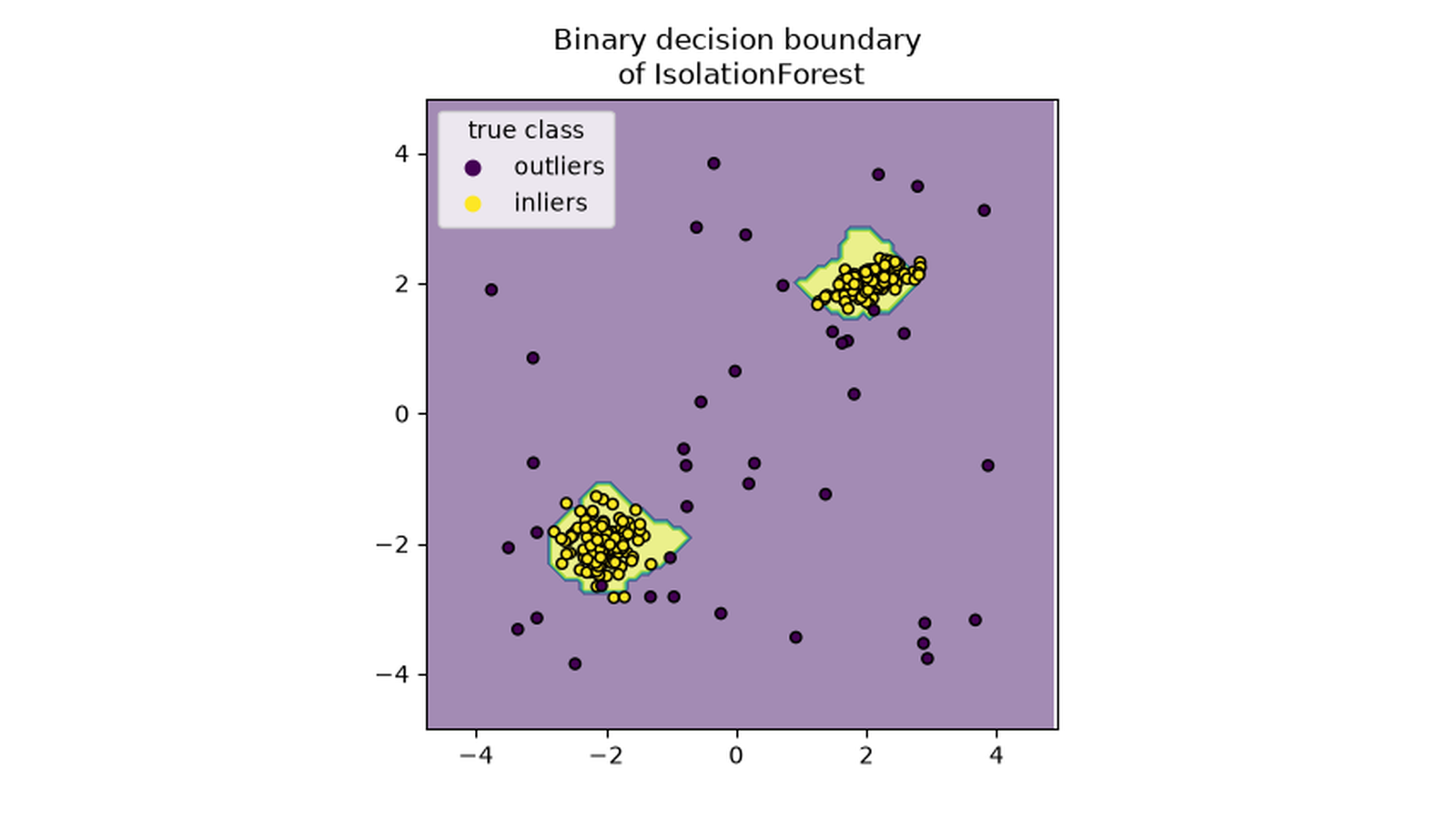
系統把一筆資料打了 0.8 分,能不能告訴同事:「這筆有八成機率異常」?先別急。Isolation Forest、Autoencoder 和 GANomaly 可以對同一筆資料給出不同尺度、甚至方向相反的分數。把分數排到前面,還不等於知道該不該發出警報。
這篇從三種打分方式出發,接著做一個可重跑的小實驗:只用正常點訓練,另留正常點選閾值,最後才用混合測試資料計算漏報與誤報。讀完後,你應該能回答:模型把什麼當成異常線索?警報閾值從哪來?這個測試到底支持了什麼?
先定義異常,再決定模型能學到什麼
「很少發生」和「需要處理」不是同一個條件。新客戶的第一次大額訂單可能少見,卻完全合理;每天固定多扣一筆小額費用可能很常見,卻需要調查。異常偵測提供的是值得進一步檢查的線索,業務規則與人工查證仍然重要。
還要區分資料來源。如果訓練資料裡已經混入少量異常,我們可能試著從整體分布找出偏離的點。如果能取得一批可信的正常樣本,則可以學正常狀態,檢查新資料是否偏離。若已經有足夠可靠的正常/異常標籤,也應把監督式分類當成候選,而不是因為題目叫「異常」就排除它。
本文的實作採第二種設定:只用正常樣本訓練。後面引用的官方 Isolation Forest 圖例則採混合資料,兩者不是同一個實驗。
這張圖也提醒我們:異常點不一定遠離每一個正常點。生成方式標成異常的點,仍可能落在正常群集附近。只看空間位置的模型,不會自動知道資料生成時的身分。
Isolation Forest:容易被隔離,是一種可用的線索
想像反覆隨機挑一個特徵,再在它的取值範圍內選一條切線,把資料分成兩邊。一筆周圍很稀疏的資料,可能只需要幾次切分就獨自留在一個節點;密集群集裡的點,通常需要更多切分。
Isolation Forest 建立很多棵這樣的樹,綜合隔離路徑的長短打分。這不是決策樹用標籤挑出最大分類增益的流程。有限樣本、樹深度與葉節點內的剩餘樣本還會影響路徑估計,不能只把分數理解成某一棵樹的整數深度。
在本文執行的 scikit-learn 1.5.1 中,score_samples 越小越偏異常;decision_function 再扣掉 offset_,預設判定的負側偏異常。我們會使用 -score_samples,把方向統一成「越大越值得檢查」,另外用校準集定閾值。
本文使用的異常分數 = -score_samples(x)
decision_function(x) = score_samples(x) - offset_

contamination="auto" 時 offset_ = -0.5
本文不使用 predict 的預設分界,另選正常校準分數的閾值。
contamination 會影響內建分界的設定方式。把它設成某個比例,並不代表模型已經從資料證明未來異常就佔那個比例,也不是把分數校準成機率。
這也是閱讀技術圖的一個習慣:先確認背景、散點、圖例和色條各來自哪個量,再討論數值代表什麼。圖看起來連續,不表示數值已具有機率意義。
Autoencoder:正常資料能重建,異常資料就一定不能嗎?
Autoencoder 先把輸入壓成表示,再用這個表示重建輸入。如果只用正常資料訓練,可以把重建誤差當作偏離正常模式的線索。二維資料的一個簡單打分方式是:先以訓練資料統計量縮放兩個特徵,再計算兩欄重建誤差的平方平均。
z = Encoder(x)
x_reconstructed = Decoder(z)
score_AE(x) = mean((x_reconstructed - x)^2)

這裡的 x 是按正常訓練資料 mean/std 縮放後的輸入。
縮放有實質影響。如果一欄以百萬元計、另一欄只在 0 到 1 之間,直接相加的誤差會被量級較大的欄位主導。用什麼特徵、怎麼縮放、如何聚合誤差,都是模型定義的一部分,應在測試前決定。
但「正常訓練」沒有保證網路只會重建正常資料。容量很大的網路可能也能重建某些異常;異常也可能位於網路學到的平滑延伸上。反過來,尚未涵蓋的正常情境,也可能有很高的重建誤差。低訓練 loss 只能說明它在訓練資料上的重建情況。
因此,不能用「訓練 loss 降了」代替異常偵測測試,也不能把重建誤差大直接解讀成某個已知故障原因。
GANomaly:把重建後的資料再編碼一次
GANomaly 是 Akcay、Atapour-Abarghouei 與 Breckon 在 2018 年提出的工作。它保留輸入到重建的流程,另外把重建結果再送入第二個 encoder,得到另一個潛在表示。比較兩個表示的差異,就多了一種異常線索。
除了表示差異,原方法的訓練還結合三個目標:判別器特徵的接近程度、輸入和重建的 contextual loss,以及兩個潛在表示的 encoder loss。它們有各自權重,不能只寫一句「加上 GAN 就會更準」。
z = Encoder_1(x)
x_reconstructed = Decoder(z)
z_reconstructed = Encoder_2(x_reconstructed)

本文概念模型的 generator objective:
feature_MSE + 50 * contextual_mean_L1 + latent_MSE

本文測試分數:mean((z - z_reconstructed)^2)
要留意論文與實作的角色。原論文訓練 encoder loss 使用 L2 表示,測試公式 Eq. 5 使用 L1;兩個式子處理不同角色,不能只因範數不同就說它們是同一個函式或必然寫錯。此次讀取的官方程式則以平方差平均作潛在分數。本文小模型明確採用 latent MSE,不能冒稱逐式重現論文。
原論文另把整批測試分數做 min-max 縮放。那會依整批測試資料的最小值、最大值改變尺度,並沒有得到校準機率。本文不使用測試集 min-max,也不把 discriminator 的 real/fake 輸出當作異常機率。
用另一批正常資料,把分數變成警報
先為每種模型保留一批沒有參與訓練的正常資料,計算正常分數分布,再按事先決定的規則取閾值。例如本文選第 95 百分位,超過才發報。這是經驗規則:它提供可檢查的警報定義,沒有自動保證未來正常資料恰好有 5% 被誤報。
threshold = np.quantile(normal_calibration_scores, 0.95, method="higher")
flagged = test_scores > threshold
這裡有 40 筆校準分數,higher 選排序後第 39 筆;嚴格大於閾值,實際只有最高的 1 筆超過。樣本少、分數有重複或正常分布改變,都會使觀察比例與直覺上的「5%」不同。這不是涵蓋率保證。
校準集也不能無限次充當調參試場。若用它挑模型、架構、特徵或分位數,這些都是選擇的一部分,需要保留最終測試來評估整套決策。本文固定三種方法與規則後,才對最終測試計分,沒有按測試答案重新挑閾值。
有異常標籤時,可以研究不同閾值下的 Precision、Recall 或成本;缺少異常標籤時,僅靠正常分數無法知道會漏掉多少種類的異常。這是評估資訊的限制,換一個深度模型名稱不會消除它。
實作:相同資料分工,三種分數各自校準
這次使用自行設定的二維點,不下載業務資料。第一欄沿 −1 到 1 展開,第二欄是第一欄的線性與正弦組合,再加固定的小擾動。異常點是在第二欄交替加減 0.8,刻意偏離這條關係。
| 用途 | 筆數 | 是否用來更新模型或定閾值 |
|---|---|---|
| 正常訓練 | 160 | 更新模型;計算兩欄 mean 與母體 std |
| 正常校準 | 40 | 模型不更新,分別決定三個閾值 |
| 最終正常測試 | 40 | 只計算誤報與正確不發報 |
| 最終位移測試 | 20 | 只計算偵測與漏報 |
四組點用不同的取樣位置產生;這是固定的教學設計,沒有聲稱它們是獨立同分布抽樣、盲測或外部驗證。所有縮放量只來自 160 個正常訓練點。
Isolation Forest 使用 80 棵樹、max_samples=128、random_state=7。AE 採 2→8→1→8→2,中間 Tanh;E-D-E 概念模型多一個 2→8→1 encoder,另設小判別器。AE、generator 和 discriminator 各實際更新 500 次。這個固定預算不是收斂證明,也沒有讓不同模型獲得相等的最佳化難度。
執行環境是 Python 3.10.12、NumPy 1.26.3、scikit-learn 1.5.1、PyTorch 2.3.1+cu118;網路實際使用 CPU、float64、單執行緒。版本是本次驗證環境,並非最新版本宣稱。來源 gallery 則是此次取得的官方文件版本,不能把來源圖當成本次程式輸出。
將下面完整程式另存為 anomaly_scores_and_thresholds.py。已安裝 Python 的環境中,可先建立虛擬環境並安裝相同套件版本;PyTorch 的套件來源與 CPU/CUDA 安裝選項須依你的作業系統選擇,本文沒有測試所有平台。
numpy==1.26.3
scikit-learn==1.5.1
torch==2.3.1
將上面的版本清單另存為 requirements.txt。以下是 WSL/Linux 的建立與執行方式;若系統缺少 venv 模組,需先依 Python 安裝方式補齊。套件安裝依當時平台取得的發行檔而定;本文實際執行核對的是前述已安裝環境,沒有聲稱重新測過所有下載來源。
python3 -m venv .venv
source .venv/bin/activate
python -m pip install -r requirements.txt
python anomaly_scores_and_thresholds.py > stdout.json
執行完成應得到含 training_record 與三組 results 的 JSON。可先檢查每組 TP+FP+FN+TN 是否為 60,再對照下方表格。若安裝到不同版本或換平台,不承諾最後一位小數或整份檔案逐 byte 一致。
"""Actual normal-only fits and separate normal calibration on a hand-set 2D toy.

EDE is a small encoder-decoder-encoder / feature-matching teaching model, not
a replication of GANomaly's image architecture or benchmark. No external data.
"""
import json
import platform

import numpy as np
import sklearn
import torch
from sklearn.ensemble import IsolationForest
from torch import nn


UPDATES = 500
SEED = 7


def normal_points(count, phase):
    t = -1 + 2 * (np.arange(count) + phase) / count
    disturbance = 0.02 * (np.arange(count) % 5 - 2)
    return np.column_stack((t, 0.5 * t + 0.15 * np.sin(3 * t) + disturbance))


class Autoencoder(nn.Module):
    def __init__(self):
        super().__init__()
        self.encoder = nn.Sequential(nn.Linear(2, 8), nn.Tanh(), nn.Linear(8, 1))
        self.decoder = nn.Sequential(nn.Linear(1, 8), nn.Tanh(), nn.Linear(8, 2))

    def forward(self, x):
        return self.decoder(self.encoder(x))


class EDE(nn.Module):
    def __init__(self):
        super().__init__()
        self.encoder1 = nn.Sequential(nn.Linear(2, 8), nn.Tanh(), nn.Linear(8, 1))
        self.decoder = nn.Sequential(nn.Linear(1, 8), nn.Tanh(), nn.Linear(8, 2))
        self.encoder2 = nn.Sequential(nn.Linear(2, 8), nn.Tanh(), nn.Linear(8, 1))

    def forward(self, x):
        z = self.encoder1(x)
        reconstructed = self.decoder(z)
        return reconstructed, z, self.encoder2(reconstructed)


class Discriminator(nn.Module):
    def __init__(self):
        super().__init__()
        self.features = nn.Sequential(nn.Linear(2, 8), nn.Tanh(), nn.Linear(8, 4), nn.Tanh())
        self.head = nn.Linear(4, 1)

    def forward(self, x):
        return self.head(self.features(x)).squeeze(-1)


def ede_losses(generator, discriminator, x):
    reconstructed, z, z_reconstructed = generator(x)
    feature = nn.functional.mse_loss(discriminator.features(reconstructed),
                                     discriminator.features(x).detach())
    contextual = nn.functional.l1_loss(reconstructed, x)
    latent = nn.functional.mse_loss(z_reconstructed, z)
    return feature, contextual, latent


def loss_record(generator, discriminator, x):
    with torch.no_grad():
        a, c, e = ede_losses(generator, discriminator, x)
    return {"feature_MSE": float(a), "contextual_L1_mean": float(c),
            "latent_MSE": float(e), "weighted_generator_objective": float(a + 50*c + e)}


def fit_networks(x):
    torch.manual_seed(SEED)
    autoencoder = Autoencoder().double()
    ae_optimizer = torch.optim.Adam(autoencoder.parameters(), lr=0.01)
    ae_initial = float(nn.functional.mse_loss(autoencoder(x), x).detach())
    for _ in range(UPDATES):
        ae_optimizer.zero_grad()
        loss = nn.functional.mse_loss(autoencoder(x), x)
        loss.backward()
        ae_optimizer.step()
    ae_final = float(nn.functional.mse_loss(autoencoder(x), x).detach())

    torch.manual_seed(SEED)
    generator, discriminator = EDE().double(), Discriminator().double()
    g_optimizer = torch.optim.Adam(generator.parameters(), lr=0.002, betas=(0.5, 0.999))
    d_optimizer = torch.optim.Adam(discriminator.parameters(), lr=0.002, betas=(0.5, 0.999))
    initial = loss_record(generator, discriminator, x)
    for _ in range(UPDATES):
        d_optimizer.zero_grad()
        with torch.no_grad():
            reconstructed = generator(x)[0]
        real_loss = nn.functional.binary_cross_entropy_with_logits(
            discriminator(x), torch.ones(len(x), dtype=torch.float64))
        fake_loss = nn.functional.binary_cross_entropy_with_logits(
            discriminator(reconstructed), torch.zeros(len(x), dtype=torch.float64))
        (0.5 * (real_loss + fake_loss)).backward()
        d_optimizer.step()
        # D weights stay fixed in this phase; gradients still pass through D to G.
        for parameter in discriminator.parameters():
            parameter.requires_grad_(False)
        g_optimizer.zero_grad()
        feature, contextual, latent = ede_losses(generator, discriminator, x)
        (feature + 50 * contextual + latent).backward()
        g_optimizer.step()
        for parameter in discriminator.parameters():
            parameter.requires_grad_(True)
    final = loss_record(generator, discriminator, x)
    autoencoder.eval()
    generator.eval()
    discriminator.eval()
    return autoencoder, generator, {"AE_initial_training_MSE": ae_initial,
        "AE_final_training_MSE": ae_final, "EDE_initial_training_losses": initial,
        "EDE_final_training_losses": final, "AE_updates": UPDATES,
        "generator_updates": UPDATES, "discriminator_updates": UPDATES,
        "parameters": {"autoencoder": sum(p.numel() for p in autoencoder.parameters()),
                       "EDE_generator": sum(p.numel() for p in generator.parameters()),
                       "discriminator": sum(p.numel() for p in discriminator.parameters())}}


def evaluate_scores(name, calibration, scores, labels):
    # Freeze the model-specific cutoff using normal calibration points only.
    threshold = float(np.quantile(calibration, 0.95, method="higher"))
    flagged = scores > threshold
    positive = labels == 1
    tp = int(np.sum(flagged & positive))
    fp = int(np.sum(flagged & ~positive))
    fn = int(np.sum(~flagged & positive))
    tn = int(np.sum(~flagged & ~positive))
    return {"model": name, "normal_calibration_scores": calibration.tolist(),
        "threshold": threshold, "threshold_rule": "np.quantile(normal_calibration, .95, method='higher'); flag score > threshold",
        "normal_calibration_flagged": int(np.sum(calibration > threshold)),
        "test_scores": scores.tolist(), "test_flagged": flagged.astype(int).tolist(),
        "TP": tp, "FP": fp, "FN": fn, "TN": tn,
        "TPR": tp / (tp + fn), "FPR": fp / (fp + tn),
        "precision": tp / (tp + fp) if tp + fp else None}


def main():
    torch.set_num_threads(1)
    torch.use_deterministic_algorithms(True)
    training = normal_points(160, 0.5)
    calibration = normal_points(40, 0.25)
    normal_test = normal_points(40, 0.75)
    abnormal_test = normal_points(20, 0.5)
    abnormal_test[:, 1] += np.where(np.arange(20) % 2 == 0, 0.8, -0.8)
    testing = np.vstack((normal_test, abnormal_test))
    labels = np.r_[np.zeros(40, dtype=int), np.ones(20, dtype=int)]
    center, scale = training.mean(axis=0), training.std(axis=0, ddof=0)
    train_scaled = (training - center) / scale
    calibration_scaled = (calibration - center) / scale
    test_scaled = (testing - center) / scale
    forest = IsolationForest(n_estimators=80, max_samples=128, random_state=SEED,
                             contamination="auto", n_jobs=1).fit(train_scaled)
    autoencoder, generator, training_record = fit_networks(
        torch.tensor(train_scaled, dtype=torch.float64))

    def score_models(values):
        x = torch.tensor(values, dtype=torch.float64)
        with torch.no_grad():
            reconstructed = autoencoder(x)
            _, z, z_reconstructed = generator(x)
            return {"isolation_forest": -forest.score_samples(values),
                "autoencoder_reconstruction_MSE": ((reconstructed-x)**2).mean(dim=1).numpy(),
                "EDE_latent_MSE": ((z-z_reconstructed)**2).mean(dim=1).numpy()}

    calibration_scores, test_scores = score_models(calibration_scaled), score_models(test_scaled)
    rows = [evaluate_scores(name, calibration_scores[name], test_scores[name], labels)
            for name in calibration_scores]
    for row in rows:
        assert np.isfinite(row["normal_calibration_scores"]).all()
        assert np.isfinite(row["test_scores"]).all()
        assert row["TP"] + row["FP"] + row["FN"] + row["TN"] == 60
    print(json.dumps({"scope": "Hand-set 2D manifold and displaced points; actual normal-only fits. "
        "EDE teaching architecture uses feature-MSE +50*contextual-L1 +latent-MSE, "
        "latent-MSE score like the retrieved official code, not exact paper equations/image replication.",
        "versions": {"python": platform.python_version(), "numpy": np.__version__,
            "sklearn": sklearn.__version__, "torch": torch.__version__},
        "device": "cpu", "dtype": "float64 for networks", "seed": SEED,
        "sizes": {"normal_training": 160, "normal_calibration": 40,
                  "normal_test": 40, "abnormal_test": 20},
        "train_only_mean": center.tolist(), "train_only_population_std": scale.tolist(),
        "training_record": training_record, "test_labels": labels.tolist(), "results": rows,
        "hypothetical_base_rate_example_not_model_measurement": {
            "assumed_TPR": 0.9, "assumed_FPR": 0.05, "assumed_prevalence": 0.01,
            "precision": 0.9*0.01/(0.9*0.01+0.05*0.99)},
        "limits": ["No abnormal labels or final test scores choose thresholds or training settings.",
            "The held-out normal quantile is empirical, not a probability or coverage guarantee.",
            "Deterministic synthetic sets are not iid external validation or a blind benchmark.",
            "Different raw score scales cannot be compared as probabilities.",
            "IF predict/auto offset is not used: the cutoff is calibrated on negative score_samples.",
            "EDE is a small fully connected concept model, not GANomaly image-benchmark reproduction.",
            "Paper training L2/inference L1 and retrieved software's MSE differ; no test-set minmax used.",
            "One seed and fixed budgets do not establish convergence or general model ranking.",
            "The artificial test anomaly fraction 20/60 is not a real operational base rate."]},
        ensure_ascii=False, indent=2))


if __name__ == "__main__":
    main()
訓練目標下降,與真的抓到異常要分開看
這次 AE 訓練 MSE 從 1.289475 降到 0.005472;E-D-E 的加權 generator 目標從 49.086323 降到 2.998599。後者包含會隨判別器訓練而改變的特徵,不能把兩者數值直接當成同一個量尺比較。
按各自正常校準分數選閾值後,最終測試得到以下結果。表中 precision 是「發報後有多少真為這次設定的異常」,不是每筆分數的機率。
- 0.596892
- 12
- 2
- 8
- 38
- 60%
- 5%
- 85.71%
- 0.014732
- 20
- 1
- 0
- 39
- 100%
- 2.5%
- 95.24%
- 0.049620
- 1
- 2
- 19
- 38
- 5%
- 5%
- 33.33%
例如 Isolation Forest 抓到 20 個位移點中的 12 個,漏掉 8 個;40 個正常點中有 2 個發報,因此這次 precision 是 12/(12+2)。三個閾值的尺度不同,不能因 0.014732 比 0.596892 小,就說 AE 比較保守或比較有信心。
E-D-E 在這次小實驗中漏掉大部分位移點。這個結果應保留下來:訓練目標下降,沒有保證選定的 latent score 能分開最終正常與異常。它不支持宣稱「加上第二個 encoder 必然變好」,也不支持反過來宣稱 GANomaly 對所有影像都沒用。
同樣地,AE 的 100% recall 只來自 20 個刻意沿同一欄位移的點。這個異常生成方式、單一種子、固定更新次數與二維網路,都限制了結論。需要改進時,應開新一輪訓練/驗證規劃,保留新的最終測試;不能反覆看這張表挑到滿意,再繼續稱它為未看過的測試。
稀有異常的困難,常在警報量而不是模型名稱
再看一個與上表分開的假設算例:一萬筆資料只有 1% 真異常;系統抓到其中 90%,正常資料的誤報率是 5%。它會抓到 90 筆異常,同時對 9,900 筆正常中的 495 筆發報,總共 585 筆警報。發報 precision 約為 15.38%。
假設異常比例 = 0.01
假設 TPR = 0.9,FPR = 0.05
Precision = (0.9 * 0.01) / (0.9 * 0.01 + 0.05 * 0.99)
          ≈ 0.153846
這不是本文三個模型的測量結果。它只說明:即使抓到九成異常,低基準率下仍可能讓調查團隊面對大量誤報。本文人工測試有 20/60 為異常,不能把表中的 precision 原封不動搬到只有 1% 異常的場景。
準備導入時,可以先列出每一天最多能處理幾筆警報、漏掉哪類事件最昂貴,以及誰能回填可靠標籤。評估要報每類異常的漏報情況、正常誤報率、precision 與實際警報量,不能只留下整體準確率或 AUC。
也要讓時間順序、設備或使用者群組符合實際部署:同一設備近乎重複的紀錄若同時進入訓練與測試,表現可能過度樂觀。正常模式改變時,舊閾值會失效;重訓、重校準與重新評估要有獨立資料及真實回饋。
選模型時,先問資料與評估能支持到哪裡。Isolation Forest 適合當作容易建立的表格資料候選;AE 和 GANomaly 類方法提供不同的表示與重建線索,但增加的結構也帶來訓練、打分與驗證選擇。有用的成果是讓每個警報能被定義、被查核並持續改善。
來源、圖片與重現材料
方法依據包括 GANomaly 原論文 arXiv v3、原作者官方程式、Isolation Forest 官方示例、Precision-Recall 官方示例 與 Jia/Liu 的架構說明原文 Figure 1。原 GANomaly 論文圖像不在本次轉載範圍;官方軟體 MIT 不用來推論論文圖像授權。
官方文件的 圖片使用說明 明示文件生成圖片可依 BSD-3-Clause 使用;這與輸入資料的條件分開。Frontiers Figure 1 依該文 CC BY 4.0 署名引用。
Iris 上游署名:R. A. Fisher,1936,UCI Iris 資料頁,DOI 10.24432/C56C76,CC BY 4.0。來源圖使用 scikit-learn 的 load_iris;API 文件 明示自 0.20 修正兩個資料點,與 R 的版本相同、與 UCI 的版本不同。此處未宣稱兩者逐列或逐 byte 相同,也沒有重跑來源 LinearSVC 圖例。
以下保留完整圖像/資料署名與 BSD 條款:
IMAGE AND DATA ATTRIBUTION

Figures 1–3 and Figure 5 are generated images from the official scikit-learn 1.9.1 documentation. Creator: The scikit-learn developers. Source pages: https://scikit-learn.org/stable/auto_examples/ensemble/plot_isolation_forest.html and https://scikit-learn.org/stable/auto_examples/model_selection/plot_precision_recall.html. The scikit-learn documentation FAQ states that its repository images and images generated in its documentation may be used under the BSD 3-Clause License. Figures 1–3 and Figure 5 are copied byte-for-byte from those pages.

Figure 4 is adapted from Figure 1 by Haoyang Jia and Wenfen Liu, “Anomaly detection in images with shared autoencoders,” published 2023-01-04, DOI: https://doi.org/10.3389/fnbot.2022.1046867, licensed CC BY 4.0: https://creativecommons.org/licenses/by/4.0/. The full source drawing was decoded from WebP and encoded as PNG; the mobile companion shows the full image followed by two overlapping source crops, resized for reading. This later simplified explanatory diagram represents the GANomaly method; the original method is by Samet Akcay, Amir Atapour-Abarghouei, and Toby P. Breckon, “GANomaly: Semi-Supervised Anomaly Detection via Adversarial Training” (2018): https://arxiv.org/abs/1805.06725. The original paper figure is not reproduced.

The precision-recall example uses scikit-learn’s `load_iris` data. Dataset credit: R. A. Fisher, “Iris” (1936), UCI Machine Learning Repository, DOI: https://doi.org/10.24432/C56C76. UCI lists the hosted Iris dataset under CC BY 4.0: https://creativecommons.org/licenses/by/4.0/. Scikit-learn documents that its v0.20+ packaged copy corrects two points according to Fisher and matches R, not the current UCI file. This corrected version and difference are disclosed; it is not claimed to be byte-identical to the current UCI download. The chart is a binary Iris/LinearSVC illustration, not anomaly-detection performance.

BSD 3-Clause License text (scikit-learn documentation images):

BSD 3-Clause License

Copyright (c) 2007-2026 The scikit-learn developers.
All rights reserved.

Redistribution and use in source and binary forms, with or without
modification, are permitted provided that the following conditions are met:

* Redistributions of source code must retain the above copyright notice, this
  list of conditions and the following disclaimer.

* Redistributions in binary form must reproduce the above copyright notice,
  this list of conditions and the following disclaimer in the documentation
  and/or other materials provided with the distribution.

* Neither the name of the copyright holder nor the names of its
  contributors may be used to endorse or promote products derived from
  this software without specific prior written permission.

THIS SOFTWARE IS PROVIDED BY THE COPYRIGHT HOLDERS AND CONTRIBUTORS "AS IS"
AND ANY EXPRESS OR IMPLIED WARRANTIES, INCLUDING, BUT NOT LIMITED TO, THE
IMPLIED WARRANTIES OF MERCHANTABILITY AND FITNESS FOR A PARTICULAR PURPOSE ARE
DISCLAIMED. IN NO EVENT SHALL THE COPYRIGHT HOLDER OR CONTRIBUTORS BE LIABLE
FOR ANY DIRECT, INDIRECT, INCIDENTAL, SPECIAL, EXEMPLARY, OR CONSEQUENTIAL
DAMAGES (INCLUDING, BUT NOT LIMITED TO, PROCUREMENT OF SUBSTITUTE GOODS OR
SERVICES; LOSS OF USE, DATA, OR PROFITS; OR BUSINESS INTERRUPTION) HOWEVER
CAUSED AND ON ANY THEORY OF LIABILITY, WHETHER IN CONTRACT, STRICT LIABILITY,
OR TORT (INCLUDING NEGLIGENCE OR OTHERWISE) ARISING IN ANY WAY OUT OF THE USE
OF THIS SOFTWARE, EVEN IF ADVISED OF THE POSSIBILITY OF SUCH DAMAGE.
留言0
登入後就能留言。
登入