
每天一筆訂單量,原本只有日期和數字。若想把它交給 Random Forest,模型卻需要一張特徵表:每列一個要預測的目標,旁邊放可以幫忙的資訊。
最自然的資訊就是最近發生的事:昨天多少、上週同一天多少、最近七天平均多少。但只要視窗往右多放一天,模型可能把今天的答案當成今天的特徵。另一個更隱蔽的問題是:訓練表每列都有昨天的真值,實際一次預測十四天時,第二天開始的「昨天」卻還沒發生。
上一篇先建立時間切分、季節基線與 ARIMA 的觀念。本篇把這條時間邊界落到資料表與程式:先核每列特徵,再實際訓練森林,最後逐步把自己的預測接回去。讀者會看見驗證選出的模型,到了下一段未必仍勝過簡單基線。
一列資料,要先決定是在預測哪一天
以每日資料為例,假設我們在第 t 天開始前預測當天的訂單,昨日觀測已經結算可用。最基本的監督式資料列可以寫成:
target(t)   = y(t)
lag1(t)     = y(t-1)
lag7(t)     = y(t-7)
rolling7(t) = [y(t-7) + ... + y(t-1)] / 7
target 是答案;其餘三欄都在這個答案發生以前。lag 代表滯後多少筆觀測,rolling 則把一段歷史壓成統計量。前者保留指定位置,後者提供最近水準的摘要。它們不是必須搭配特定模型的專用欄位,同一張表也能交給線性回歸或梯度提升樹。
官方範例使用小時資料,所以除了前一小時、前一天,還會放前一週等欄位。本文自己的實作則是每日人工資料,只使用 lag1、lag7、rolling7,加上七個星期位置指示欄。不要把外部圖的小時 lag 直接照搬成每日序列的天數。
第一個可訓練的目標在 index 7,因為它之前剛好有七個觀測。以下來自本文實際輸出,省略七個日曆指示欄,數值只在表中四捨五入:
| target index | 當天 target | lag1 | lag7 | rolling7 |
|---|---|---|---|---|
| 7 | 45.7 | 58.6 | 43.0 | 52.442857 |
| 8 | 47.8 | 45.7 | 47.1 | 52.828571 |
| 9 | 49.9 | 47.8 | 51.2 | 52.928571 |
例如 index 7 的平均只取 index 0–6,不包含 45.7 這個當天答案。到了 index 8,昨天的 45.7 已經成為歷史,因此可以出現在 lag1。相同數字能不能使用,取決於預測發生的時間,而不是它曾經被叫作 target 就永遠不能再用。
shift 移的是數值對齊,不能只改日期標籤
在 pandas,建立昨天值的常見寫法是把序列向後移一列:
lag1 = y.shift(1)
lag7 = y.shift(7)
不指定 freq 時,正的 periods 會讓較早的數值對齊到較晚的列,開頭留下缺值。原本 index 0 的觀測,現在成為 index 1 這列的歷史特徵。
要分清的是,shift(freq="D") 主要移動時間索引標籤,並不是同一個「把昨日數值接到今天 target」的操作。日期看起來晚了一天,不代表特徵與答案就已正確配對。合併回目標表以前,仍要核對索引、頻率與真正可用的歷史。
負的 shift 常用來建立未來目標,例如想把 t+7 的答案放到 t 這列;如果把它錯放進特徵,就直接看到了未來。是否安全要看欄位用途:未來值可以是訓練 label,卻不能是當時拿不到的輸入,而且訓練截止日之後的 label 也不能混進 fit。
rolling 的右邊界,決定有沒有把答案平均進去
直接寫 y.rolling(7).mean(),預設會包含當列的 y(t)。若這列要預測的正是 y(t),就已把未知答案放進特徵。本文先 shift,再 rolling:
rolling7 = y.shift(1).rolling(7).mean()
這樣 index t 的右邊界停在 t−1,往左共七筆。先把公式寫出來,再核程式,會比只記住某一串 pandas 語法可靠。
固定筆數視窗與時間長度視窗也不同。rolling(7) 看七筆;有 datetime index 時,rolling("7D") 看七天範圍,若有缺日或同一天多筆,包含的筆數就可能不同。整數視窗預設需要完整 window 數量的有效觀測才輸出;時間長度視窗的 min_periods 預設則不同,不能看到同樣寫「七」就當成相同特徵。
本文的每日資料沒有缺日,rolling 的 min_periods 沿用整數視窗預設七筆,因此前七列沒有完整 lag7/rolling7,直接移除。這是在承認歷史不足,不是把缺值解釋成零需求。若真實資料的中段有缺值,還要另決定缺值是漏報、停業還是真正零值,不能直接補零或從未來回填。
center=True 或向前看的 window 尤其要小心:它們可用於事後平滑與描述,卻可能把預測時間點後的觀測放進統計量。整張表算得出數字,不代表當時算得出來。
程式另放了一個可檢查的反例:只把 y[10] 增加 70,index 10 的安全特徵完全不變,因為它們最多看到 index 9。未 shift 的七日平均卻增加 10,正好是 70/7。這比單看最終分數,更直接暴露 target 是否進入視窗。
排好時間還不夠:要排對群組與可用時間
單一序列以時間排序後 shift,通常很直觀。若資料變成多家門市,直接對整欄 shift,某家店的第一天可能接到上一家店最後一天的數字。應先按「門市、時間」排序,再在各門市內形成自己的歷史;rolling 同樣不能跨越群組邊界。
還要分清「觀測日期」與「拿到資料的日期」。假設昨日訂單要到今天中午才結算,早上九點預測時就不能用昨日最終值。此時合法的 lag 可能必須更長,或改用當時可取得的速報版本。後來修正的歷史資料,也不能冒充當年當時看到的版本。
日曆則是另一種欄位。星期、已知假日通常可以預先取得;未來真實雨量或未來實際價格調整則要看它們何時確定。本文七個 weekday 指示欄只是 index 對七取餘數的人造週期位置,沒有對應真實公曆日期,也沒有為真實資料處理假日。
因此,每新增一欄,都可以問同一個具體問題:如果把時間停在這次預測的起點,這個值真的已存在嗎?不只答案欄需要問,日後的聚合、填補、標準化與特徵選擇也一樣。
訓練時看過昨日真值,十四天後的昨日卻可能是預測
假設最後知道的是第 T 天,要一次交付 T+1 到 T+14。第一天的 lag1 可以用真實 y(T),但第二天的 lag1 就需要 y(T+1),而它此時還不知道。
最直接的處理方式是 recursive:先用一個單步模型預測第一天,再把這個預測當成歷史接回去,產生第二天的特徵。七日平均與 lag7 也要跟著這條更新後的歷史走;不能只有 lag1 接預測,其他欄位仍偷用完整測試真值。
起點已知:... y(T-1), y(T)
預測一步:ŷ(T+1)
接回歷史:... y(T), ŷ(T+1)
再算特徵 → 預測 ŷ(T+2)
重複,直到 ŷ(T+14)
這也帶來訓練與部署的落差:訓練列裡的 lag 多半是真值,遞迴後段則混入模型自己的預測,誤差可能透過特徵繼續傳遞。但不是每一步都必然更差,也不是誤差一定單調增加;要按實際 horizon 評估。
其他常見策略解決的方式不同:
- 單步模型反覆預測,接回自己的輸出
- 模型可共用;需要逐步計算特徵,可能受回饋誤差影響
- 分別訓練第 1、2、…、14 步模型
- 不必把前一步預測當輸入;多個模型與各 horizon 的標籤要管理
- 一個模型同時輸出十四個目標
- 可一起建模多步關係;模型需支援向量輸出,訓練樣本要有完整目標範圍
Direct 的十四個模型不必分享完全相同的誤差結構;multi-output 也不是把 recursive 的結果換個格式輸出。兩者建立訓練 label 時,都要確保 label 的最晚時間沒有超過訓練截止日。模型數量、單次模型複雜度、資料量與服務方式一起決定成本,不能只用「一個模型」就斷言最便宜。
本文只實作 recursive 與另一個明確分開的每日 one-step 協定,沒有訓練 direct 或 multi-output 模型,也不宣稱哪一種策略普遍較準。
先讓候選接受同一個十四天預測任務
把序列變成表格,不代表它就變成可以任意隨機切的獨立資料。相鄰列有大量重疊歷史,隨機切分還可能讓較晚的資料參與訓練,再回頭評估較早的時段。
本文使用兩個擴張起點驗證,然後留下最後一段。索引從零開始,lag7 使第一個訓練 target 是 index 7:
| 區段 | fit 的 target 索引 | 從起點一次預測 |
|---|---|---|
| 驗證一 | 7–125 | 126–139,共十四點 |
| 驗證二 | 7–139 | 140–153,共十四點 |
| 最後評估 | 7–153 | 154–167,共十四點 |
兩個候選是先定週期七的季節 naive,以及固定參數森林。季節 naive 把最後七天重複兩輪;森林每一步則重算 lag1、lag7、rolling7 和七個日曆指示欄。兩者都只有起點之前的真實歷史,段內不取得新觀測。
森林用 40 棵樹、最大深度 6、每葉至少 3 筆、seed 7、單一 job。沒有用最後區段調這些值。樹可以利用非線性與特徵交互作用,但本例森林的每棵樹在葉節點仍輸出訓練目標的平均,不能因此期待它自動把持續成長向訓練範圍外延伸。
完整資料是 168 點人工訊號,包含每步 0.1 的成長、七步週期形狀與五步確定擾動,沒有抽樣真實門市資料。資料形狀、週期與候選都是教學預設,不是盲測或隨機搜尋的勝出組合。
完整程式與實際輸出
這支程式已在下列既有環境實際執行,輸出包含完整人工序列、前幾列特徵、每折十四點預測、最後選擇與 one-step 協定:
Python 3.10.12
numpy 1.26.3
pandas 2.2.2
scikit-learn 1.5.1
把下方完整程式存成檔案,已有對應套件的環境可執行:
python3 lag_rolling_forecasts.py > stdout.json
依賴版本可記成以下 requirements。本文核對的是現有環境,不宣稱在所有平台全新安裝都已驗證。外部文件使用 scikit-learn 1.5.2、pandas 2.2.3,與本次執行版本分開列出。
numpy==1.26.3
pandas==2.2.2
scikit-learn==1.5.1
"""Original synthetic teaching example: safe lag features and recursive forecasts.

Daily observations arrive without delay. Fixed-origin 14-day forecasts never
receive the intermediate actuals. A separately labelled one-step protocol does.
"""
import json
import platform

import numpy as np
import pandas as pd
import sklearn
from sklearn.ensemble import RandomForestRegressor


PERIOD = 7
HORIZON = 14
PATTERN = (-6, -3, 0, 2, 5, 11, 8)
DISTURBANCE = (-1, 0, 1, 0, -1)
SERIES = [50 + 0.1 * t + PATTERN[t % PERIOD] + DISTURBANCE[t % 5]
          for t in range(168)]
FEATURES = ["lag1", "lag7", "rolling7"] + [f"weekday{k}" for k in range(7)]
CANDIDATES = ("seasonal_naive", "random_forest")


def feature_table(history):
    """Row t predicts y[t]; every target-derived feature ends at t-1."""
    y = pd.Series(history, dtype=float)
    table = pd.DataFrame({"target": y, "lag1": y.shift(1),
                          "lag7": y.shift(7),
                          "rolling7": y.shift(1).rolling(7).mean()})
    for k in range(7):
        table[f"weekday{k}"] = (table.index % 7 == k).astype(int)
    return table.dropna()


def next_features(history):
    """History may contain previous predictions during recursive deployment."""
    t = len(history)
    assert t >= 7
    return [history[-1], history[-7], float(np.mean(history[-7:]))] + [
        int(t % 7 == k) for k in range(7)]


def fit_forest(history):
    table = feature_table(history)
    model = RandomForestRegressor(n_estimators=40, max_depth=6,
                                  min_samples_leaf=3, random_state=7, n_jobs=1)
    model.fit(table[FEATURES].to_numpy(), table["target"].to_numpy())
    return model


def forecast(history, name, model=None):
    """Only the observed prefix is supplied; recursively append own predictions."""
    prefix = list(history)
    if name == "seasonal_naive":
        return [prefix[-PERIOD + h % PERIOD] for h in range(HORIZON)]
    assert name == "random_forest" and model is not None
    predicted = []
    for _ in range(HORIZON):
        value = float(model.predict([next_features(prefix)])[0])
        predicted.append(value)
        prefix.append(value)
    return predicted


def mae(truth, predicted):
    return float(np.mean(np.abs(np.asarray(truth) - np.asarray(predicted))))


def rounded(values):
    return np.round(values, 8).tolist()


def main():
    validation = []
    for origin in (126, 140):
        history = SERIES[:origin]
        model = fit_forest(history)
        for name in CANDIDATES:
            predicted = forecast(history, name, model)
            validation.append({"origin": origin, "training_target_indices": [7, origin - 1],
                "forecast_indices": [origin, origin + HORIZON - 1], "model": name,
                "prediction": rounded(predicted), "truth": rounded(SERIES[origin:origin + HORIZON]),
                "MAE": mae(SERIES[origin:origin + HORIZON], predicted)})
    scores = {name: float(np.mean([row["MAE"] for row in validation
                                  if row["model"] == name])) for name in CANDIDATES}
    selected = min(CANDIDATES, key=lambda name: (scores[name], CANDIDATES.index(name)))
    # Freeze selection before reading final-block errors.
    origin = 154
    model = fit_forest(SERIES[:origin])
    final = []
    for name in CANDIDATES:
        prediction = forecast(SERIES[:origin], name, model)
        final.append({"model": name, "selected_using_validation_only": name == selected,
            "prediction": rounded(prediction), "truth": rounded(SERIES[origin:]),
            "MAE": mae(SERIES[origin:], prediction)})

    # Different information contract: true past is revealed before each next day.
    # Same already-fitted forest, no refits; this is not a fixed-origin result.
    one_step = [float(model.predict([next_features(SERIES[:t])])[0])
                for t in range(origin, len(SERIES))]

    table = feature_table(SERIES[:origin])
    alignment_error = max(abs(a - b) for t in table.index
                          for a, b in zip(table.loc[t, FEATURES], next_features(SERIES[:t])))
    assert alignment_error < 1e-12
    # Perturb y[10] itself: correctly shifted features for target 10 stay fixed;
    # the unshifted rolling mean includes the unavailable target and changes.
    changed = SERIES.copy()
    changed[10] += 70
    safe = feature_table(SERIES).loc[10, FEATURES].to_numpy()
    safe_changed = feature_table(changed).loc[10, FEATURES].to_numpy()
    assert np.array_equal(safe, safe_changed)
    unsafe_delta = float(pd.Series(changed).rolling(7).mean()[10]
                         - pd.Series(SERIES).rolling(7).mean()[10])
    assert abs(unsafe_delta - 10) < 1e-12
    print(json.dumps({"scope": "Hand-set 168-point daily teaching signal; actual fitted forest, "
        "not an external benchmark. Calendar known, observations available without delay.",
        "versions": {"python": platform.python_version(), "numpy": np.__version__,
            "pandas": pd.__version__, "sklearn": sklearn.__version__},
        "series": rounded(SERIES), "features": FEATURES,
        "first_three_training_rows": table.head(3).reset_index(names="target_index").to_dict("records"),
        "feature_alignment_max_error": alignment_error,
        "target_perturbation_check": {"index": 10, "target_increase": 70,
            "shifted_features_unchanged": True, "unshifted_rolling_mean_change": unsafe_delta},
        "validation": validation, "mean_validation_MAE": scores,
        "selected_before_final_evaluation": selected,
        "final_fixed_origin": {"origin": origin, "training_target_indices": [7, 153],
            "forecast_indices": [154, 167], "horizon": HORIZON, "results": final},
        "different_one_step_observed_history_protocol": {
            "refit": False, "predictions": rounded(one_step), "MAE": mae(SERIES[origin:], one_step),
            "scope": "Each prediction gets actual observations through t-1. "
                     "Not available to the fixed-origin 14-day forecast; not a rival model score."},
        "limits": ["The pattern, candidate hyperparameters and folds were fixed for teaching.",
            "Validation training prefixes overlap; folds are not independent samples.",
            "No random-split comparison, prediction intervals or general model ranking.",
            "Tree forecasts can fail under extrapolation or distribution shift.",
            "Real panels require grouping; delayed values require availability-time handling."]},
        ensure_ascii=False, indent=2))


if __name__ == "__main__":
    main()
保存輸出中的驗證平均如下。它是在兩個驗證起點的相同十四步 MAE 上選模型,最後區段不參與選擇:
{
  "mean_validation_MAE": {
    "seasonal_naive": 1.514285714285713,
    "random_forest": 1.4619162286126577
  },
  "selected_before_final_evaluation": "random_forest"
}
| 候選 | 驗證一 MAE | 驗證二 MAE | 驗證平均 | 最後十四點 MAE |
|---|---|---|---|---|
| 季節 naive | 1.564286 | 1.464286 | 1.514286 | 1.292857 |
| Random Forest | 1.370979 | 1.552854 | 1.461916 | 1.448743 |
驗證選了森林,最後卻是季節基線較好。這個結果應該保留,不能看完最後分數再宣稱自己原本選的是基線。兩個驗證起點也有大量重疊訓練資料,不是兩份獨立資料集,不能僅憑這一點小差異做顯著性或一般優劣推論。
最後一段前兩步能看見遞迴的差異:起點預測 index 154 約 61.262047,接著 index 155 約 61.388879。第二步用的 lag1 是前一步預測 61.262047,而不是後來看到的真值 58.4。到第二週,lag7 也開始包含第一週的預測;程式用一份只含已知歷史與自身預測的 prefix,讓所有視窗一起遵守這個邊界。
每天拿到新真值,是另一份預測契約
如果實際工作是每天早上重新預測今天,昨日真值在那之前已經到達,就可以使用更近期的實際歷史。這是合法的 one-step observed-history 任務;它與年初一次交付未來十四天,是不同服務需求。
程式最後另用同一個已擬合森林、不重新 fit,每天取得截至 t−1 的真實觀測後預測 t。它的 MAE 約 1.522394,本例反而比十四步 recursive 的 1.448743 略差。因此不能把「能拿到更多真歷史」改寫成「對任何固定模型一定更準」。模型如何切分特徵空間、預測偏差怎麼累積,都會影響這一段的實際結果。
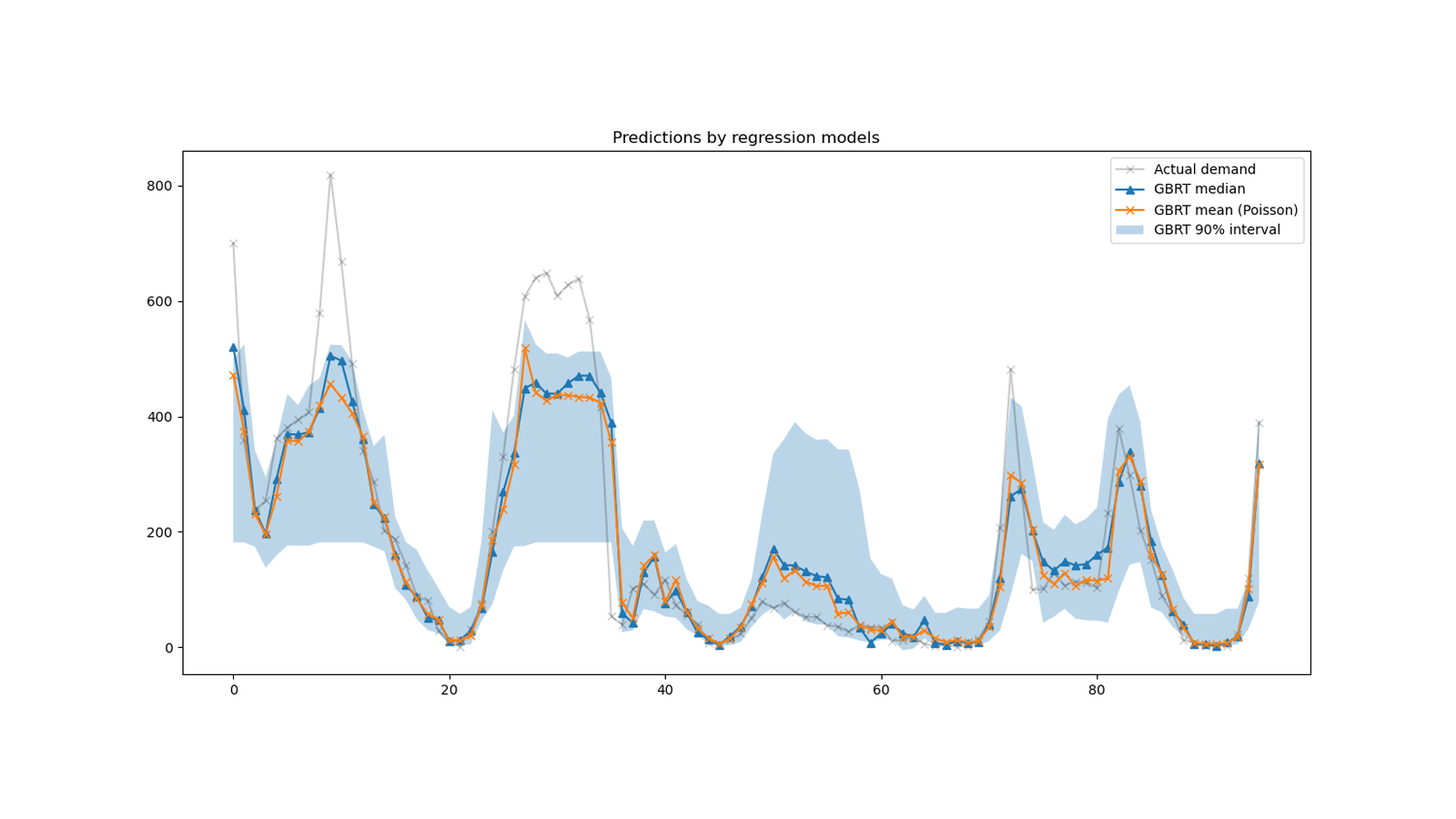
對這類圖先問清楚資訊契約,再看線條貼不貼近。若模型在每個測試列都取得實際的前一小時值,就不能把一整段圖當成「從最左端起點一次預測到最右端」的成果。圖上的區間也需要另做實證覆蓋檢查,不能只因名稱寫 90% 就認為已校準。
對一個新的門市任務,最有用的檢查是沿著一筆具體預測往回追:這列答案是哪天?每欄的最後觀測時間是哪天?十四步的後段是拿預測還是真值重算?然後才比較模型。只要這些時間角色清楚,lag 與 rolling 才是在把歷史交給模型,而不是把答案藏進表格。
來源、資料脈絡與圖像授權
本文的原創部分是人工 168 點序列、十個特徵的逐列檢查、target 擾動反例、森林固定起點遞迴與 one-step 的分開實作,以及兩次驗證後保留最後排名反轉的結果。外部圖為來源文件輸出,沒有冒充本站模型或資料重跑。
- scikit-learn:完整 lagged-feature 範例、時間切分圖與程式、TimeSeriesSplit 說明、1.5.2 BSD 3-Clause 原版。來源範例用 Polars、HistGradientBoostingRegressor 與小時 BikeSharing 資料;本文用 pandas、RandomForestRegressor 與人工每日序列,不能混成同一次實驗。
- pandas 2.2.3:DataFrame.shift 的原文與輸出表、DataFrame.rolling 的原文與輸出表、BSD 3-Clause 原版。
- Bike Sharing 原資料:UCI dataset/DOI 10.24432/C5W894,creator Hadi Fanaee-T,UCI 記錄明示 CC BY 4.0。OpenML v2 metadata 記錄 Joaquin Vanschoren 的類別文字、溫度/風速反正規化與欄位改名等整理;本文未驗目前 UCI 與這份 OpenML 處理版逐列、逐 byte 相同,不把 metadata 的 Public 欄位當成授權名稱。
- 資料引用依原記錄保留 Fanaee-T、Gama 的 Event labeling combining ensemble detectors and background knowledge(2013)。此處作資料來源 citation,不宣稱本文重現該論文方法或讀完全文。
以下保留選用圖的完整署名、變更及兩份 BSD 授權全文。資料來源 CC BY 4.0 與軟體/文件 BSD 的範圍分開說明。
# DS61 source image credits and reuse notices

The following source-derived images accompany this article. The credits, changes and applicable license notices are retained below. The article source list provides clickable links to the original documentation and dataset records.

## scikit-learn 1.5.2 documentation figures and output

- `fig-01-timeseries-split.png`: scikit-learn developers, generated TimeSeriesSplit example, [documentation page](https://scikit-learn.org/1.5/modules/cross_validation.html#time-series-split), [source PNG](https://scikit-learn.org/1.5/_images/sphx_glr_plot_cv_indices_013.png). Synthetic generated indices; four expanding splits. Reused without pixel changes.
- `fig-02-lagged-feature-table.png` and `fig-02-mobile-lagged-feature-table.png`: scikit-learn developers, [Lagged features for time series forecasting](https://scikit-learn.org/1.5/auto_examples/applications/plot_time_series_lagged_features.html), v1.5.2. The source table is rendered from the example's `lagged_df.tail(10)` output. The full table had to be captured in two horizontal browser-scroll states because the official page clips its 14-column output in the content viewport. The source code and table are retained; the two captures are stitched in original column order, and the mobile derivative first shows the complete image, then stacks five complete original column groups, each proportionally enlarged to 620 pixels wide with LANCZOS. The target-count column is repeated only for row identification and is not a predictor input. No table values, labels or row order are changed.
- `fig-06-official-forecast.png` and `cover.png`: same scikit-learn example and authors. `fig-06` is the original source PNG, reused without pixel changes. `cover.png` is the complete source plot fitted proportionally on a white 1600×900 canvas without added text or marks. It reports the last 96 rows of the first TimeSeriesSplit fold (all_splits[0], 3,000 test rows); it is not the DS61 practice output or a calibration guarantee.

The Bike Sharing data underlying the scikit-learn example is credited separately from the scikit-learn documentation: UCI record [Bike Sharing Dataset](https://archive.ics.uci.edu/dataset/275/bike+sharing+dataset), creator Hadi Fanaee-T, [CC BY 4.0](https://creativecommons.org/licenses/by/4.0/). The associated paper is Hadi Fanaee-T and João Gama, “Event labeling combining ensemble detectors and background knowledge,” DOI [10.1007/s13748-013-0040-3](https://doi.org/10.1007/s13748-013-0040-3); João Gama is an associated-paper coauthor, not a name in the UCI record's Creators field. The example retrieves OpenML `Bike_Sharing_Demand` version 2 (data id 42712). OpenML metadata identifies the UCI source and credits Joaquin Vanschoren for cleanup: replacing category labels, reversing temperature/wind normalization, and changing feature names. No row-by-row byte comparison was performed, and no byte-exact UCI identity is claimed. The OpenML `Public` field is not represented as a license.

## pandas 2.2.3 documentation outputs

- `fig-03-shift-lag-table.png`: pandas documentation contributors, [`DataFrame.shift`](https://pandas.pydata.org/pandas-docs/version/2.2.3/reference/api/pandas.DataFrame.shift.html), version 2.2.3; source code/output example screenshot, not an independent original figure. Right-side page whitespace is cropped; complete code, headers, dates, NaN and all five output rows are retained.
- `fig-04-rolling-row-window.png` and `fig-05-rolling-time-window.png`: pandas documentation contributors, [`DataFrame.rolling`](https://pandas.pydata.org/pandas-docs/version/2.2.3/reference/api/pandas.DataFrame.rolling.html), version 2.2.3; source code/output example screenshots, not independent original figures. Right-side page whitespace is cropped; complete code, headers, dates where present, NaN and all five output rows are retained. The examples use synthetic data. These unshifted rolling examples include the current row and illustrate window/min_periods behavior, not the shifted forecasting features in this article.

## Full license texts

The following notices are copied verbatim from scikit-learn 1.5.2 and pandas 2.2.3 project license files.

### scikit-learn 1.5.2 BSD 3-Clause License

BSD 3-Clause License

Copyright (c) 2007-2024 The scikit-learn developers.
All rights reserved.

Redistribution and use in source and binary forms, with or without
modification, are permitted provided that the following conditions are met:

* Redistributions of source code must retain the above copyright notice, this
  list of conditions and the following disclaimer.

* Redistributions in binary form must reproduce the above copyright notice,
  this list of conditions and the following disclaimer in the documentation
  and/or other materials provided with the distribution.

* Neither the name of the copyright holder nor the names of its
  contributors may be used to endorse or promote products derived from
  this software without specific prior written permission.

THIS SOFTWARE IS PROVIDED BY THE COPYRIGHT HOLDERS AND CONTRIBUTORS "AS IS"
AND ANY EXPRESS OR IMPLIED WARRANTIES, INCLUDING, BUT NOT LIMITED TO, THE
IMPLIED WARRANTIES OF MERCHANTABILITY AND FITNESS FOR A PARTICULAR PURPOSE ARE
DISCLAIMED. IN NO EVENT SHALL THE COPYRIGHT HOLDER OR CONTRIBUTORS BE LIABLE
FOR ANY DIRECT, INDIRECT, INCIDENTAL, SPECIAL, EXEMPLARY, OR CONSEQUENTIAL
DAMAGES (INCLUDING, BUT NOT LIMITED TO, PROCUREMENT OF SUBSTITUTE GOODS OR
SERVICES; LOSS OF USE, DATA, OR PROFITS; OR BUSINESS INTERRUPTION) HOWEVER
CAUSED AND ON ANY THEORY OF LIABILITY, WHETHER IN CONTRACT, STRICT LIABILITY,
OR TORT (INCLUDING NEGLIGENCE OR OTHERWISE) ARISING IN ANY WAY OUT OF THE USE
OF THIS SOFTWARE, EVEN IF ADVISED OF THE POSSIBILITY OF SUCH DAMAGE.

### pandas 2.2.3 BSD 3-Clause License

BSD 3-Clause License

Copyright (c) 2008-2011, AQR Capital Management, LLC, Lambda Foundry, Inc. and PyData Development Team
All rights reserved.

Copyright (c) 2011-2023, Open source contributors.

Redistribution and use in source and binary forms, with or without
modification, are permitted provided that the following conditions are met:

* Redistributions of source code must retain the above copyright notice, this
  list of conditions and the following disclaimer.

* Redistributions in binary form must reproduce the above copyright notice,
  this list of conditions and the following disclaimer in the documentation
  and/or other materials provided with the distribution.

* Neither the name of the copyright holder nor the names of its
  contributors may be used to endorse or promote products derived from
  this software without specific prior written permission.

THIS SOFTWARE IS PROVIDED BY THE COPYRIGHT HOLDERS AND CONTRIBUTORS "AS IS"
AND ANY EXPRESS OR IMPLIED WARRANTIES, INCLUDING, BUT NOT LIMITED TO, THE
IMPLIED WARRANTIES OF MERCHANTABILITY AND FITNESS FOR A PARTICULAR PURPOSE ARE
DISCLAIMED. IN NO EVENT SHALL THE COPYRIGHT HOLDER OR CONTRIBUTORS BE LIABLE
FOR ANY DIRECT, INDIRECT, INCIDENTAL, SPECIAL, EXEMPLARY, OR CONSEQUENTIAL
DAMAGES (INCLUDING, BUT NOT LIMITED TO, PROCUREMENT OF SUBSTITUTE GOODS OR
SERVICES; LOSS OF USE, DATA, OR PROFITS; OR BUSINESS INTERRUPTION) HOWEVER
CAUSED AND ON ANY THEORY OF LIABILITY, WHETHER IN CONTRACT, STRICT LIABILITY,
OR TORT (INCLUDING NEGLIGENCE OR OTHERWISE) ARISING IN ANY WAY OUT OF THE USE
OF THIS SOFTWARE, EVEN IF ADVISED OF THE POSSIBILITY OF SUCH DAMAGE.
留言0
登入後就能留言。
登入