
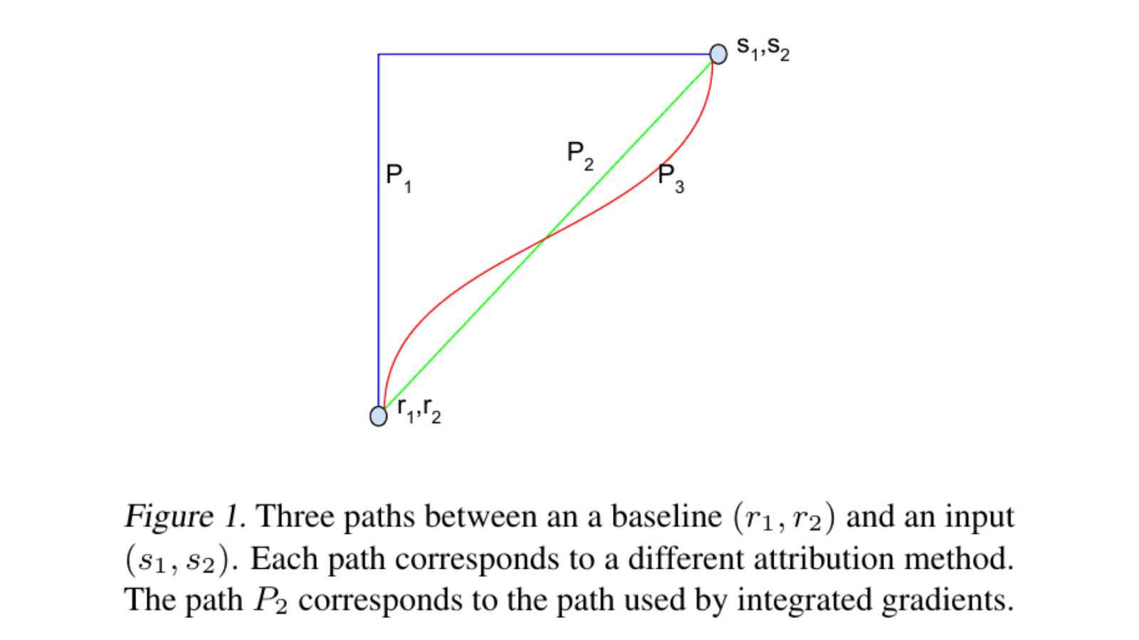
把某個特徵遮掉,模型分數沒有變;對那個特徵求梯度,結果也等於零。能不能因此說,模型完全不依賴它?
先看你做了哪一種測試。單次遮擋比較指定替換前後的輸出,梯度看目前位置附近的微小變動;兩者都不必然回答「從某個基準走到這筆輸入,輸出的差額要怎麼分」。Integrated Gradients 沿選定路徑累積梯度,Layer-wise Relevance Propagation 則沿網路連線按指定規則分配 relevance。名稱不同,問題與前提也不同。
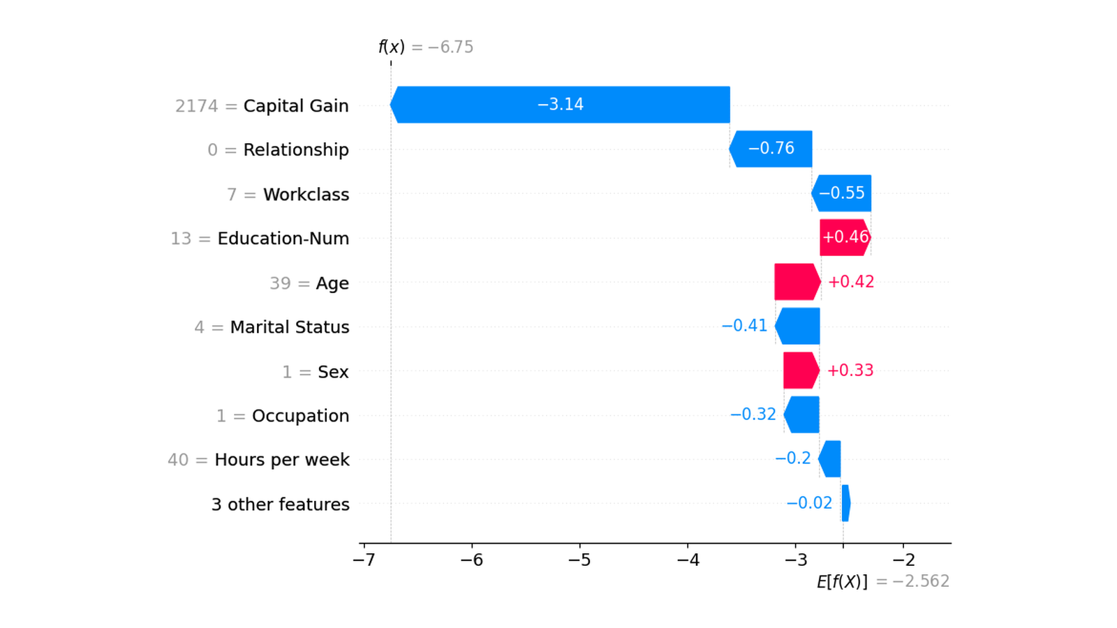
上一篇 SHAP已看過,背景與缺失特徵的定義會改變歸因。本篇把問題轉到可微函數與神經網路,先用遮擋、梯度與平坦區理解差別,再手算 IG 與具體 LRP 規則。五張原圖提供來源方法與研究情境;完整 Python 小例只用手設函數,沒有訓練影像模型或執行解釋套件。
先固定目標分數,再決定要問哪一種變化
解釋前,先選定一個標量輸出 f(x)。對分類器而言,這可能是某類別的 logit、機率或其他分數;它們的尺度與梯度不同,不能混加。如果只想知道模型為何支持某類,應固定該類別,而不是在每個擾動點重新挑最高分的類別,最後卻把結果當成同一個函數。
接著分辨四種問題:
這些量不必一致。分歧可能來自替換值、基準、飽和、特徵交互作用或規則本身,不一定是其中一支程式算錯。反過來,兩張熱圖看起來相近,也不能直接證明它們回答了相同問題。
遮擋:一次替換造成的落差,不一定能相加
對第 i 個特徵做替換,可以計算:
drop_i = f(x) − f(把第i個特徵換成指定值後的x)
影像裡,替換單位可以是一個像素、一塊區域或 superpixel;填值可能是零、灰色、均值或模糊後的值。文字裡,刪詞與換成佔位符也不相同。單位和替換方法都會改變你實際查詢的輸入。
例如另設一個兩特徵函數:
f(x1,x2) = x1 + 2x2 + x1x2
目標 (1,1):分數4
只把x1換成0:(0,1),分數2,drop1=2
只把x2換成0:(1,0),分數1,drop2=3
兩個 drop 相加是 5,大於原分數 4。因為兩次替換都包含交互作用消失的效果,這部分被重複計入了。單獨遮擋的落差不是自動滿足加總守恆的特徵分配。
替換後的資料也可能不自然。黑色方塊可能引入強烈邊緣,刪詞可能破壞語法;分數下降可能同時反映資訊移除與人工輸入造成的分布差異。這不代表不能做遮擋,而是回報時必須說清楚它測的是哪種替換,不能把結果直接叫成現實世界的因果效果。
梯度:在這裡怎麼變,不等於一路怎麼走到這裡
輸入梯度的第 i 維是 ∂f/∂x_i。在可微位置、變動足夠小時,它描述每單位輸入變化帶來的局部輸出變化。若換了輸入單位或前處理尺度,梯度數字也會改;它不是沒有單位的通用重要性。
gradient×input 再把梯度乘上 x_i。對零截距線性函數,這能對上各項輸出;對一般非線性函數,它仍只是當下梯度乘數值,不會因此自動變成精確輸出分解。若熱圖再取絕對值,正負方向也會被合併;亮度高並不直接等於「支持這個類別」。
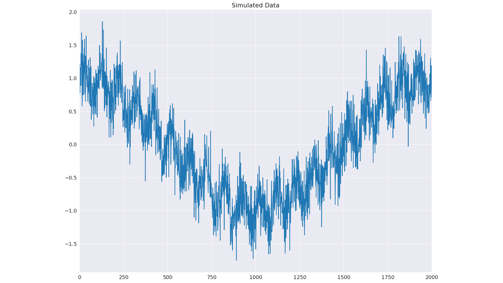
圖中的問題是:當下的變化方向,能不能代表相對某個邊界的解釋?這與「梯度有沒有算對」不同。另一個常見落差來自飽和:函數在終點附近已經變平,即使從基準走來的過程曾經大幅上升,終點梯度仍可能很小。
這條曲線的斜率只描述沿所選插值方向的輸出變化,單靠曲線不能讀出每個像素的偏導數。也不要把「沿這個方向變平」讀成「模型一路都沒有用到輸入」。接下來用一個能完整手算的飽和函數,另外逐維計算梯度,把差別拆開。
Integrated Gradients:沿選定路徑,把梯度累積起來
IG 需要原輸入 x,以及 baseline b。標準直線路徑與第 i 維歸因為:
路徑:gamma(alpha) = b + alpha × (x−b),alpha從0到1

IG_i = (x_i−b_i) × integral from0to1:
                       ∂f(b+alpha×(x−b)) / ∂x_i  d alpha
這不是只對終點求一次梯度。它在路徑上多個位置求梯度,再乘上該維從 baseline 到輸入的變化量。baseline 的數字要以模型真正接收的空間定義;前處理後的零向量,不一定對應原始黑色影像,也不自動表示「什麼資訊都沒有」。
考慮這個手設函數:
s = x1 + 2x2
f(x1,x2) = ReLU(s) − ReLU(s−1)

s≤0:f=0
0<s<1:f=s
s≥1:f=1
目標是 (1,1),f=1;零基準 (0,0) 的 f=0。在目標附近已飽和,所以梯度與 gradient×input 都是 (0,0)。只把 x1 換成零,s=2、f 仍為1;只把 x2 換成零,s=1、f 也仍為1,因此兩個遮擋 drop 都是0。剩餘特徵各自都足以維持輸出,並不表示它們在整個函數中完全沒作用。
沿零基準直線,路徑是 (alpha,alpha),s=3alpha。只有前 1/3 路徑處於上升區,其梯度為 (1,2);之後梯度為0。因此:
IG1 = 1 × [1 × (1/3)] = 1/3
IG2 = 1 × [2 × (1/3)] = 2/3
總和 = 1 = f(1,1)−f(0,0)
零梯度、零單特徵替換 drop,以及非零 IG 可以同時成立。它們衡量的是不同的變化,不能只拿誰的數字較大就判斷誰比較正確。
完整性與數值誤差,要和解釋品質分開
在能使用路徑上的微積分基本定理的前提下,IG 的 completeness 表示:
sum_i IG_i = f(x)−f(b)
本例是連續、有限分段線性的函數,能在各段直接積分,再把結果接起來。這裡不把「幾乎處處可微」單獨當成對任意函數都足夠的保證,也不需要在 ReLU 折點替某個特定導數約定賦予積分質量。
實作時通常用有限點近似積分。本篇使用 midpoint,並把「歸因總和減去輸出差」印成 delta:
| 同一零基準路徑的 midpoint 步數 | IG 總和 | delta |
|---|---|---|
| 8 | 1.125 | 0.125 |
| 32 | 1.03125 | 0.03125 |
| 128 | 1.0078125 | 0.0078125 |
| 512 | 1.001953125 | 0.001953125 |
| 2048 | 1.00048828125 | 0.00048828125 |
程式另外算 300 步,得到 (1/3,2/3)、delta=0。這個步數恰好讓分段位置與積分格子對齊;不能因此宣稱任何模型用 300 步都會精確。表格也只展示本例這些格點的收斂情況,不保證任意函數每加一步誤差都下降。
delta 小,是必要時可用的數值檢查,但正負誤差可能抵銷,不能單憑總和吻合就證明每維歸因都已精確,更不能證明 baseline 合理、解釋符合人類語意或具有因果意義。
換一個 baseline,分配的差額也會換
保持模型與目標 (1,1) 不變,改用 b=(0.1,0)。baseline 的輸出已經是0.1,所以現在要分配的差額是0.9,而不是1。
路徑 = (0.1+0.9alpha, alpha)
s(alpha) = 0.1+2.9alpha
到alpha=9/29時,s=1,此後飽和

IG1 = 0.9 × 9/29 = 81/290 ≈ 0.279310345
IG2 = 2 × 9/29 = 18/29 ≈ 0.620689655
總和 = 0.9
300 步 midpoint 的實際輸出是 (.279,.62),總和 .899、delta 約 −.001。既顯示了換 baseline 的分配差別,也顯示同樣 300 步不再恰好精確。
baseline 不是一個只為讓程式能跑的參數。如果輸入某維剛好等於 baseline,同維的差值因子為0,其 IG 就會是0;這說的是相對此基準沒有變化,不保證該值對模型毫無含義。以黑色影像作基準,也可能讓本來就是黑色的物體區域沒有這種差值。
Distill 的研究比較了常數、模糊、噪聲與基準分布,討論各自對 missingness 的假設;沒有給出適用所有任務的唯一最佳選項。本篇不重現其照片或整套評估,只保留圖 2 的自有曲線。使用真實模型時,應一起回報 baseline、輸出尺度、前處理、路徑與積分設定;路徑中間點也可能離開訓練資料分布,不能因為採直線就忽略這件事。
LRP:先選 relevance 傳播規則,再談守恆
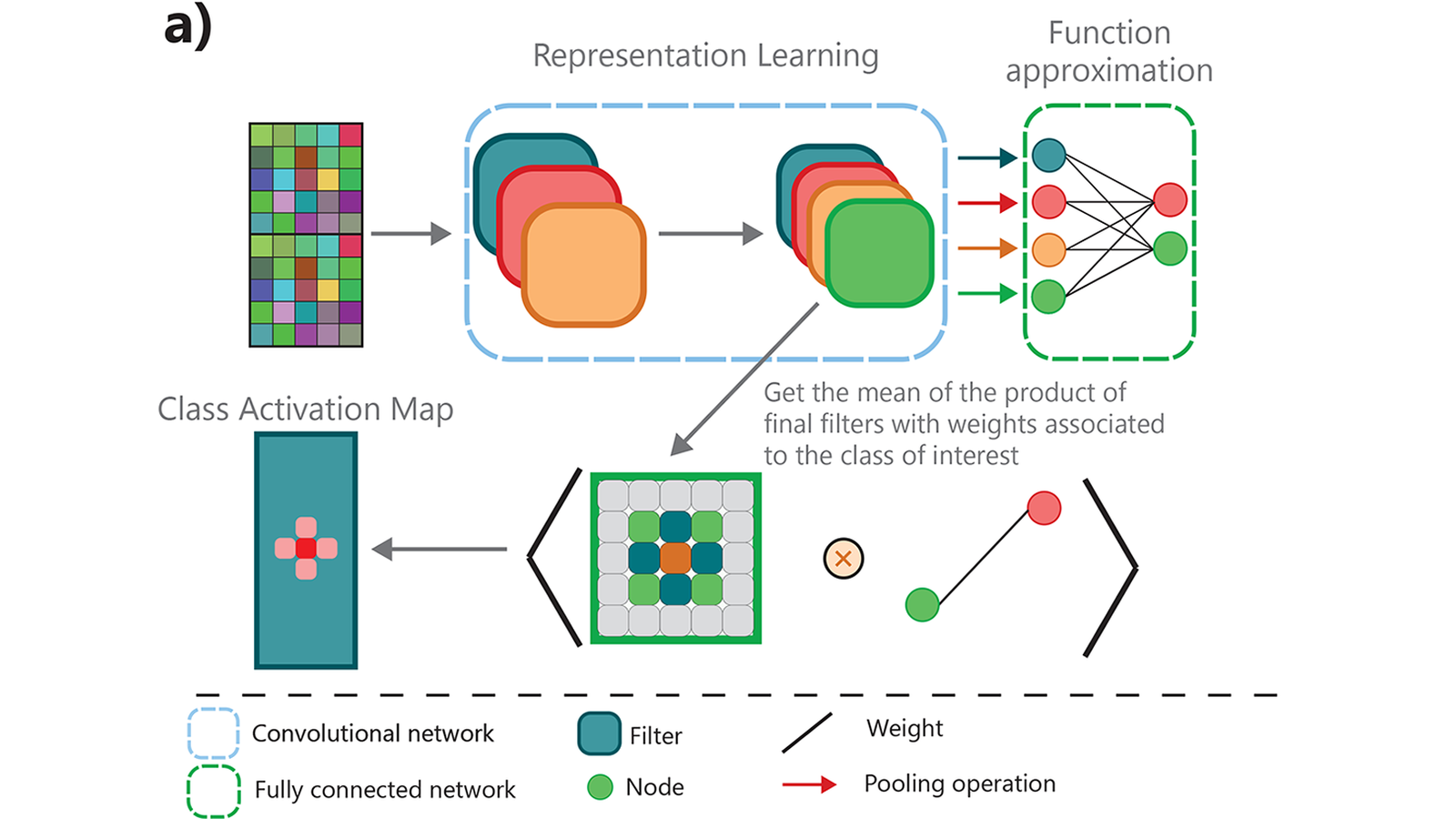
IG 沿基準到輸入的路徑積分;LRP 從網路某個輸出的 relevance 出發,往輸入方向分配。它利用各層的連線與前向活動,但反向傳的是定義好的 relevance 訊息,不必然是普通反向傳播的導數。
原文先給 relevance 與訊息的限制條件,再討論可採用的分配算法;不是只憑一張網路圖就唯一決定輸入分數。以最簡單的正權、非負輸入、無 bias、分母非零情況為例,可以採用:
z_ij = a_i × w_ij
R_(i←j) = z_ij / sum_k z_kj × R_j
R_i = sum_j R_(i←j)
這是本篇實作的簡化 z-rule。對每個上層節點 j,把 R_j 按各個前向輸入項 z_ij 的比例分配,比例加起來為1,就能在這一層保留 relevance 總量。若分母為0,就不能照此式硬除;遇到負項、bias 或不同激活函數,也需要重新交代規則與適用前提。
單層例子是 input=(3,1)、weights=(2,1),輸出7。兩個前向項是6與1;從 R_out=7 開始,按6/7、1/7分配,得到 relevance=(6,1)。這是刻意簡單的正權線性情況,不是所有 LRP 都會得到同一種比例。
分兩層傳一次:epsilon 穩定項會吸收什麼?
另設一個便於逐步核對的兩層正權、無 bias 網路:
input = (1,2)
h1 = 1×1 + 2×1 = 3
h2 = 1×2 + 2×1 = 4
output = 2h1 + 1h2 = 10
這是另一個函數,不是先前的飽和模型,不能拿兩者的數值當成方法排名。兩個 hidden 值均為正;即使中間放 ReLU,也會原樣通過。本程式直接算這些明定的和,不呼叫神經網路框架。
先從輸出 relevance=10 分到 h1/h2,得到6/4。再往下分:
| 上層 relevance | 給 input1 的訊息 | 給 input2 的訊息 |
|---|---|---|
| h1:6 | (1/3)×6=2 | (2/3)×6=4 |
| h2:4 | (2/4)×4=2 | (2/4)×4=2 |
| 各輸入收到的總量 | 4 | 6 |
總量4+6=10。在這個特例裡,它也等於有效線性函數 (4x1+3x2) 的 gradient×input;不能據此說兩種方法在任意網路都相同。
若分母很小,比例可能很不穩定。原 LRP 論文也討論 epsilon 穩定項,並明確指出 bias 與穩定項可能吸收 relevance。本例所有分母為正,加入 epsilon=1/2 後的規則簡化為:
R_(i←j) = z_ij / (sum_k z_kj + epsilon) × R_j
epsilon 在這裡只改 relevance 的分配,不改前向模型,也不是重新訓練的正則項。程式在兩次層間分配都加入同樣的 epsilon,沒有再分配被吸收的殘量。實際結果為:
| 規則 | hidden relevance | input relevance 總和 |
|---|---|---|
| epsilon=0 的 z-rule | (6,4) | 10 |
| 每層 epsilon=1/2 | (40/7,80/21) | 10960/1323 ≈ 8.284203 |
epsilon 版的兩個 input relevance 是 4400/1323、6560/1323,輸出10減去它們的總和,還有 2270/1323。這是此穩定規則的吸收,不是程式忘了把一個神經元算進去。
因此「LRP 必定完整分配全部輸出」不能脫離規則來說。若換成有 bias、帶符號項或其他 LRP 變體,殘量如何處理也必須重查。LRP 分配的還是選定模型輸出的 relevance,不會因為有守恆式,就升級成輸入對真實世界結果的因果效果。
完整可跑程式:核對機制,不用下載影像模型
以下程式保存的實跑環境為 Python 3.10.12,只用標準庫。它明列解析梯度,另在非折點位置用中央差分核對;沒有呼叫 autograd、Captum、IG 或 LRP 套件 API。ReLU 折點的導數在程式中約定為0,但本文使用的 midpoint 格點避開折點,積分結果不靠對折點導數的特殊取值。
將完整程式存成 explanation_mechanics.py,執行:
python3 explanation_mechanics.py
#!/usr/bin/env python3
"""Hand-specified explanation mechanics; Python standard library only.

No trained model, dataset, autograd framework, or attribution package is used.
Saturated-score comparisons use one function. LRP uses a separate, explicitly
positive, bias-free network. They are not a method-quality benchmark.
"""

from fractions import Fraction as F
import json
import math


def saturated_score(x1, x2):
    s = x1 + 2 * x2
    return max(s, 0) - max(s - 1, 0)


def saturated_gradient(x1, x2):
    """Analytic derivative off s=0,1; choose zero at the two kinks.

    The chosen midpoint grids below never hit either kink. This convention
    does not assert differentiability at the kinks or emulate an autograd API.
    """
    s = x1 + 2 * x2
    slope = 1.0 if 0.0 < s < 1.0 else 0.0
    return slope, 2.0 * slope


def midpoint_ig(baseline, target, steps):
    delta = tuple(t - b for b, t in zip(baseline, target))
    gradients = []
    for i in range(steps):
        alpha = (i + 0.5) / steps
        point = tuple(b + alpha * d for b, d in zip(baseline, delta))
        # Only this fixed toy/grid scope is supported by this script.
        s = point[0] + 2 * point[1]
        assert not math.isclose(s, 0.0, abs_tol=1e-12)
        assert not math.isclose(s, 1.0, abs_tol=1e-12)
        gradients.append(saturated_gradient(*point))
    attribution = tuple(delta[j] * sum(g[j] for g in gradients) / steps for j in range(2))
    output_change = saturated_score(*target) - saturated_score(*baseline)
    return {"steps": steps, "attribution": attribution,
            "sum": sum(attribution), "output_change": output_change,
            "completeness_delta": sum(attribution) - output_change}


def central_difference(point, coordinate, step=1e-6):
    above, below = list(point), list(point)
    above[coordinate] += step
    below[coordinate] -= step
    return (saturated_score(*above) - saturated_score(*below)) / (2 * step)


def positive_messages(inputs, weights, relevance, epsilon=F(0)):
    """Fixed positive no-bias z-rule, or positive-denominator epsilon variant.

    epsilon is added at every redistribution layer when requested. No
    residual is redistributed. This is not a general signed/bias LRP API.
    """
    if epsilon < 0 or any(v < 0 for v in (*inputs, *weights)):
        raise ValueError("This toy requires nonnegative inputs/weights/epsilon")
    terms = tuple(a * w for a, w in zip(inputs, weights))
    denominator = sum(terms, F(0)) + epsilon
    if denominator <= 0:
        raise ValueError("Positive nonzero denominator required")
    return tuple(term / denominator * relevance for term in terms)


def two_layer_lrp(epsilon):
    x = (F(1), F(2))
    # Rows correspond to the two hidden units. ReLU leaves both positive h unchanged.
    hidden_weights = ((F(1), F(1)), (F(2), F(1)))
    output_weights = (F(2), F(1))
    hidden = tuple(sum((a * w for a, w in zip(x, row)), F(0)) for row in hidden_weights)
    output = sum((h * w for h, w in zip(hidden, output_weights)), F(0))
    hidden_r = positive_messages(hidden, output_weights, output, epsilon)
    input_messages = tuple(positive_messages(x, row, r, epsilon)
                           for row, r in zip(hidden_weights, hidden_r))
    input_r = tuple(sum((messages[j] for messages in input_messages), F(0)) for j in range(2))
    return {"epsilon_at_each_layer": str(epsilon), "x": list(map(str, x)),
            "hidden_weights_rows": [list(map(str, row)) for row in hidden_weights],
            "hidden_activations": list(map(str, hidden)),
            "output_weights": list(map(str, output_weights)), "output": str(output),
            "hidden_relevance": list(map(str, hidden_r)),
            "input_messages_by_hidden": [list(map(str, row)) for row in input_messages],
            "input_relevance": list(map(str, input_r)),
            "input_relevance_float": list(map(float, input_r)),
            "input_relevance_sum": str(sum(input_r, F(0))),
            "output_minus_input_relevance_sum": str(output - sum(input_r, F(0)))}


def main():
    baseline, target = (0.0, 0.0), (1.0, 1.0)
    gradient = saturated_gradient(*target)
    ig = midpoint_ig(baseline, target, 300)
    score = saturated_score(*target)
    occlusion = tuple(score - saturated_score(*(0.0 if j == i else target[j] for j in range(2)))
                      for i in range(2))
    convergence = [midpoint_ig(baseline, target, n) for n in (8, 32, 128, 512, 2048)]
    nonzero_baseline = (0.1, 0.0)
    changed_baseline_ig = midpoint_ig(nonzero_baseline, target, 300)
    # s(alpha)=1/10+(29/10)alpha crosses 1 at alpha=9/29.
    analytic_nonzero = (F(81, 290), F(18, 29))
    fd_checks = []
    for point in ((0.25, 0.125), target):
        analytic = saturated_gradient(*point)
        finite = tuple(central_difference(point, j) for j in range(2))
        assert all(abs(a - f) < 1e-8 for a, f in zip(analytic, finite))
        fd_checks.append({"point": point, "analytic": analytic, "central_difference": finite})

    def interaction(x1, x2):
        return x1 + 2 * x2 + x1 * x2

    original = interaction(1, 1)
    interaction_drops = (original - interaction(0, 1), original - interaction(1, 0))
    one_layer_x, one_layer_w = (F(3), F(1)), (F(2), F(1))
    one_layer_r = positive_messages(one_layer_x, one_layer_w, F(7))
    z_rule, epsilon_rule = two_layer_lrp(F(0)), two_layer_lrp(F(1, 2))

    assert gradient == (0.0, 0.0) and occlusion == (0.0, 0.0)
    assert ig["attribution"] == (1 / 3, 2 / 3)
    assert abs(ig["completeness_delta"]) < 1e-12
    assert abs(convergence[-1]["completeness_delta"]) < abs(convergence[0]["completeness_delta"])
    assert abs(sum(analytic_nonzero) - F(9, 10)) == 0
    assert all(abs(a - float(b)) < 0.001 for a, b in zip(changed_baseline_ig["attribution"], analytic_nonzero))
    assert interaction_drops == (2, 3) and sum(interaction_drops) == 5 > original
    assert one_layer_r == (F(6), F(1))
    assert z_rule["hidden_relevance"] == ["6", "4"]
    assert z_rule["input_relevance"] == ["4", "6"]
    assert z_rule["input_relevance_sum"] == "10"
    assert epsilon_rule["input_relevance"] == ["4400/1323", "6560/1323"]
    assert F(epsilon_rule["input_relevance_sum"]) < F(epsilon_rule["output"])

    result = {
        "scope": "hand-set scalar mechanisms, not training/real-image attribution/causal evidence or a package benchmark",
        "saturated_function": "ReLU(x1+2*x2)-ReLU(x1+2*x2-1)",
        "saturation_zero_baseline": {"baseline": baseline, "target": target,
            "baseline_score": saturated_score(*baseline), "target_score": score,
            "analytic_target_gradient": gradient,
            "gradient_times_input": tuple(g * x for g, x in zip(gradient, target)),
            "single_feature_zero_occlusion_drops": occlusion,
            "analytic_straight_path_ig": ["1/3", "2/3"], "midpoint_ig": ig},
        "midpoint_resolution_comparison_same_zero_baseline": convergence,
        "nonzero_baseline_same_function_target": {"baseline": nonzero_baseline,
            "target": target, "baseline_score": saturated_score(*nonzero_baseline),
            "path_saturation_alpha": "9/29",
            "analytic_straight_path_ig": list(map(str, analytic_nonzero)),
            "analytic_ig_sum": str(sum(analytic_nonzero)), "midpoint_ig": changed_baseline_ig},
        "off_kink_gradient_central_difference_checks": fd_checks,
        "interaction_occlusion": {"function": "x1+2*x2+x1*x2", "target": [1, 1],
            "score": original, "single_feature_zero_occlusion_drops": interaction_drops,
            "sum_of_drops": sum(interaction_drops), "not_an_additive_decomposition": True},
        "single_positive_linear_z_rule": {"x": [3, 1], "weights": [2, 1],
            "output": 7, "relevance": list(map(str, one_layer_r))},
        "separate_two_layer_positive_no_bias_network": {"z_rule": z_rule,
            "epsilon_variant_no_residual_redistribution": epsilon_rule,
            "scope": "different function from saturated example; all weights/activations positive, no bias; epsilon=1/2 added in both layers"},
        "limits": ["all gradients are explicitly derived, not autograd",
            "straight paths and baselines are hand-chosen; not a causal intervention",
            "300 steps is exactly aligned for the zero-baseline toy; finite quadrature is not generally exact",
            "conservation of a relevance rule does not establish semantic quality or causality"]}
    print(json.dumps(result, ensure_ascii=False, indent=2))


if __name__ == "__main__":
    main()
輸出的 JSON 會列出零基準與非零基準、各步數 IG/delta、非折點梯度檢查、交互函數的遮擋落差,以及單層/兩層 relevance 訊息。LRP 部分使用 Fraction 保留精確分數,方便逐層查核;IG 部分保留浮點近似與誤差,不把小數顯示成完全精確的解析解。
真正拿模型來解釋時,先把「要解釋哪個輸出」「移除或基準代表什麼」「使用哪套規則」「做了哪些數值與穩定性檢查」講清楚。遮擋落差大、IG 相加吻合或 relevance 守恆,都只回答各自的一部分問題。解釋是否忠實、是否受人工輸入影響、是否符合使用情境,仍須以相應測試與資料評估,不能只憑熱圖漂亮或亮在物體上就下結論。
方法、原圖與實作來源
- Mukund Sundararajan、Ankur Taly、Qiqi Yan,Axiomatic Attribution for Deep Networks,PMLR 70:3319–3328,ICML 2017:IG、baseline、路徑與 completeness。本文讀前段方法/性質、path 與必要應用前提,沒有宣稱重跑所有實驗或通讀每份上游證明。Fig.1 依當屆 publication agreement 的 CC BY 4.0條件保留完整原出版引用及原 PMLR 連結;不把後來網站的通用 footer 自動當成當年授權證據。
- Sebastian Bach、Alexander Binder、Grégoire Montavon、Frederick Klauschen、Klaus-Robert Müller、Wojciech Samek,PLOS ONE 2015,e0130140:本文直接讀 relevance/message 限制、Taylor 對照、Fig.2/3/5 及多層網路方法 Eq.55–61 的必要上下文,並原生核對 Eq.56/58/59。文中簡化 z-rule/epsilon 計算有明列正權、無 bias、正分母前提,沒有重跑原文照片模型或全部實驗。原圖依文章明列的 CC BY 4.0署名。
- Pascal Sturmfels、Scott Lundberg、Su-In Lee,Visualizing the Impact of Feature Attribution Baselines,Distill,2020:本文讀完整主文至結論/related methods、所採 Figure 3 的完整 live JavaScript,以及本篇末尾的 Reuse 條款;沒有逐篇追讀全部 references 或重新跑 Inception v4。所選僅自有 Goldfinch softmax 曲線,依本篇明列的 CC BY 4.0使用,排除照片與選圖介面。這與同站 FAQ一般圖解再利用說明分開核對,不將第三方借圖一併納入。
- 本篇完整程式是手設數值機制;其實跑、輸出與解析計算,不代表取得真實影像解釋品質、方法勝負或因果效果。各圖改作與作者歸屬另列於本文圖說與來源聲明。
圖像署名與改作聲明
五組來源圖依各自明示的 CC BY 4.0 條件署名,原文與授權均在上方提供可點連結。以下保留完整圖像來源與本次改作聲明;它不把照片、第三方圖或模型結果一併納入。
# DS58 image credits and reuse notes

These illustrations reproduce the source-created diagrams and chart listed below. Their authors, individual grants and modifications are recorded here; no photograph or model/data rerun is included.

## PLOS ONE figures

Sebastian Bach et al. (2015), Figures 2, 3, and 5, “On Pixel-Wise Explanations for Non-Linear Classifier Decisions by Layer-Wise Relevance Propagation,” *PLOS ONE* 10(7): e0130140, [doi:10.1371/journal.pone.0130140](https://doi.org/10.1371/journal.pone.0130140). The article states [CC BY 4.0](https://creativecommons.org/licenses/by/4.0/). The main images are byte-copies of the complete source figures. The mobile derivatives show the complete figure first and stack complete source panels without adding marks, text, or data. The article's separate data-availability statement about some CC0 source images is not being treated as a blanket image grant.

## Integrated Gradients Figure 1

Mukund Sundararajan, Ankur Taly, and Qiqi Yan (2017), Figure 1, “Axiomatic Attribution for Deep Networks,” *Proceedings of the 34th International Conference on Machine Learning*, PMLR 70, pp. 3319–3328, [PMLR article](https://proceedings.mlr.press/v70/sundararajan17a.html). The 2017 ICML author instructions linked the contemporaneous publication-permission form. Its §2 grants CC BY 4.0 and §3 requires citation and a PMLR link. No signed author-specific form copy is claimed. The source figure and caption are cropped from the original PDF page 4; the cover fits the complete crop proportionally on white.

## Distill chart

Pascal Sturmfels, Scott Lundberg, and Su-In Lee (2020), Figure 3 chart, “Visualizing the Impact of Feature Attribution Baselines,” *Distill*, [doi:10.23915/distill.00022](https://doi.org/10.23915/distill.00022). The article-specific footer states that diagrams and text are CC BY 4.0 and excludes externally credited figures. The selected D3 chart is the authors' own visualization and has no separate third-party credit. The currently saved Distill FAQ links CC BY 2.0; this chart relies on the article-specific CC BY 4.0 statement, not on a claim about the FAQ. The selector thumbnails and photograph are excluded. The source's chart plots Goldfinch Softmax output probability against the interpolation constant in one Inception v4 example.

The mobile chart shows the whole chart first, followed by two overlapping x-range crops. The crops omit the long title and x-axis label; readers should use the whole chart for those labels and the full range. No chart values or visual marks were redrawn or changed.
留言0
登入後就能留言。
登入