
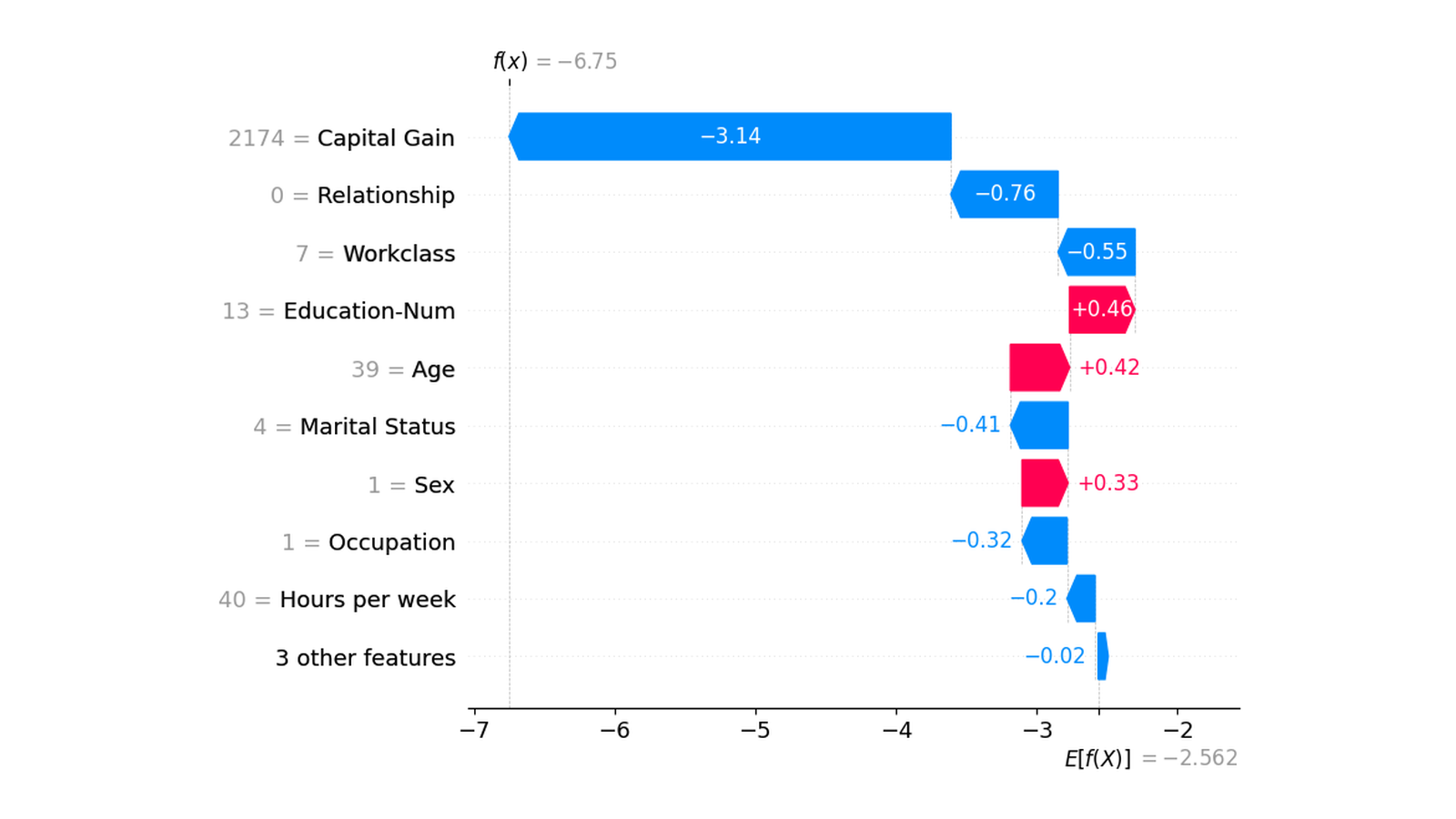
假設模型對同一個人給出一個分數。年齡、教育程度、工作時數都在輸入裡,我們想知道:哪些特徵把這次預測往上推,哪些往下拉?
要分配之前,還缺一個問題:相對於什麼?相對於輸入全零、某個參考樣本,還是某群人的平均模型輸出?基準換了,要分配的差額就變了。即使基準沒變,「只知道年齡、還不知道其他欄位」要怎麼算,也可能有不同定義。
SHAP 是 SHapley Additive exPlanations。Lundberg 與 Lee 在 2017 年把合作賽局的 Shapley 值與加法式特徵歸因連起來:對一筆預測,把相對於基準的差額分給各個特徵。本篇先用兩個特徵手算加入順序,再看背景資料與條件期望如何改變歸因,最後用官方文件的四張原圖練習讀法。
前一篇 LIME是在一個選定鄰域內擬合簡單代理模型。SHAP 也能用加法形式呈現,但它要回答的是:在已定義的特徵合作賽局裡,如何分配增量。不能只因兩張圖都顯示特徵權重,就把它們當成相同的最佳化問題。
先讀一個人的 waterfall:從基準加到這次輸出
加法式歸因最容易讀的形式是:
這次模型輸出 = 基準值 + 特徵1的歸因 + … + 特徵M的歸因
f(x*)        = phi0  + phi1          + … + phiM
x* 是正在解釋的輸入;多類分類時,還要先固定正在解釋哪個類別的輸出,不能混加不同類別的歸因。phi0 常是指定背景與解釋方式下的期望模型輸出,並不自動等於模型的截距,也不是所有人的「正常分數」。phi_i 是這次、這個輸出尺度下的特徵歸因,不是模型係數的另一個名稱。
這張來源圖的程式從 Adult 取 2000 筆,訓練 XGBoost 再產生解釋;圖是 notebook 保存的輸出,並非本站重新訓練或重新估計。例中 Capital Gain 的藍色 −3.14,表示相對於該次基準與解釋方式,它對這次 margin 有負向歸因。不能只看這一個人,就說提高資本利得必然降低收入,或這個特徵在所有人身上都同方向。
若輸出是二元分類 log-odds,可用 sigmoid 把最後總和轉成機率:
p = 1 / (1 + exp(−[phi0 + sum(phi_i)]))
不能把每個 phi_i 個別套 sigmoid,再把那些機率加在一起。sigmoid 不是線性函數;−3.14 也不是「減少 314 個百分點」。有些解釋器可以在機率尺度工作,但必須核對所解釋的 model output 與 link,不能只看資料是分類就假定所有圖都用機率。
把特徵當玩家,先定義每個組合值多少
Shapley 值的出發點,是把特徵想成合作的玩家。令 S 表示目前已知的特徵集合,v(S) 表示在這個集合下,我們定義的模型輸出。這個 v 就是賽局。
「已知某特徵」表示知道它在 x* 的值;「尚未知道」不等於把它填成數值 0,更不必然代表重新訓練一個缺該欄位的模型。填參考值、以背景資料替換、條件期望,是不同的賽局定義。
先選一個可以全部算完的例子。模型與待解釋點固定為:
f(x,z) = x + 2z + 3xz
待解釋點 (x,z) = (1,1),f(1,1) = 6

第一種賽局:只有一個背景點 (0,0)
已知的欄位固定在目標值1;未知欄位用背景值0
四個合作組合因此是:
| 已知的特徵 S | 送進模型的值 | v(S) |
|---|---|---|
| 無 | (0,0) | 0 |
| 只有 x | (1,0) | 1 |
| 只有 z | (0,1) | 2 |
| x 與 z | (1,1) | 6 |
總差額是 6−0=6。x 自己加入時只提高 1,但在 z 已知之後加入,卻提高 6−2=4;差別來自交互作用 3xz。若只看一個加入順序,就會把「後加入才出現的合作效果」偏給後加入的人。
平均所有加入順序,分配交互作用
兩個特徵只有兩種加入順序:
| 加入順序 | x 的增量 | z 的增量 |
|---|---|---|
| 先 x、再 z | 1−0=1 | 6−1=5 |
| 先 z、再 x | 6−2=4 | 2−0=2 |
| 各順序等權平均 | 2.5 | 3.5 |
所以這個賽局的結果是 0 + 2.5 + 3.5 = 6。它不是原式中一次項係數 1、2,也不是在 (1,1) 的偏導數;它平均的是所選賽局中加入玩家的輸出增量,交互作用的效果也被分配進來。這裡對稱地把交互部分的 3 分成各 1.5,因而得到 x 的 1+1.5、z 的 2+1.5。
更多特徵的標準公式,是對所有不含 i 的 S 計算「加入 i 的增量」:
phi_i = sum over S subset of F without i:
          |S|! × (M−|S|−1)! / M!
          × [v(S union {i}) − v(S)]

M:玩家數/特徵數
權重:在所有等權排列裡,恰好由S先於i出現的比例
這裡的 S 不含 i,所以是加入前後做差。不要把它和「從含 i 的集合刪掉 i」的公式混用同一個階乘係數。作者的官方 Errata已更正原 paper Eq.8 的 off-by-one;本文採用上面加入版的正確權重。
特徵很多時,組合數呈指數增加,實務上才需要抽樣近似、Kernel SHAP 的加權回歸,或利用模型結構的專用算法。不能把本例窮舉四個組合的精確答案,延伸成任何大模型解釋都已精確算完。
原始論文也把 SHAP 與加法解釋的局部準確性、missingness、consistency 連起來。局部準確性要求在正在解釋的這筆輸入相加吻合;missingness 約束可解釋表示中不存在的玩家,不是說原資料數值等於 0 就不能有歸因;consistency 要求若某玩家在所有相關組合的增量都不下降,其分配也不應下降。但「唯一」有前提:必須先固定賽局/缺失特徵操作與所用公理,不能靠特徵名字偏袒分配。作者 Errata 特別補上了論證所需的 feature anonymity 假設。它不表示所有背景、所有缺失定義與所有近似實作都會給同一份唯一正確解釋。
同一個模型,背景換了,基準與分配也會換
現在不改模型,也不改目標 (1,1),只把背景換成兩個等權點:
背景:(0,0)、(1,1),每點機率1/2
採邊際替換(marginal replacement):已知欄位固定在目標值,未知欄位從背景列取值,計算輸出後平均。有多個未知欄位時,保留它們在同一背景列的聯合取值;不是把每個缺欄分別獨立抽樣。
以「只有 x 已知」為例,兩次查詢是 f(1,0)=1、f(1,1)=6,平均 3.5。完整四值變成:
照相同順序平均,得到 phi_x=1.25、phi_z=1.75。基準加歸因仍然是 3+1.25+1.75=6,只是現在分配的是超過背景平均的 3 分,不是超過全零背景的 6 分。
這不是算法算錯,而是問題改了。選單一參考樣本、訓練母體、某個子群,可能都對應不同的比較問題。報告 SHAP 時,若只附一張圖而沒交代背景,讀者就不知道數字相對於誰。
線性模型也不能漏掉這點。在本段的邊際替換賽局下,若 f(x)=b+sum(w_j x_j),則:
phi0 = b + sum_j w_j E[X_j]
phi_j = w_j × (x*_j − E[X_j])
基準包含特徵平均,不只是 b。這也是作者 Errata 明確修正的 Linear SHAP 式子;若改成保留特徵相關資訊的條件賽局,不能直接不加前提地套同一個簡式。
條件期望換了賽局,不是換一個名稱而已
前段邊際替換把目標欄位和背景其他欄位接起來,可能造出原資料支撐之外的組合。例如背景只有 (0,0)、(1,1),程式仍會查詢 (1,0) 或 (0,1)。模型在這些位置有函數值,不代表資料真的觀察過這些組合。
另一種定義是 observational conditional expectation:只平均符合「已知欄位等於目標值」的背景資料。
v_cond(S) = E[f(X) | X_S = x*_S]
在這個兩點背景裡,知道 x=1,就只剩 (1,1);知道 z=1,也只剩同一點。因此 v(空)=3、v({x})=6、v({z})=6、v({x,z})=6,平均分配得到各 1.5。
把三種結果並列就很清楚:
| 同一模型與同一目標 | 基準 | phi_x | phi_z | 最後輸出 |
|---|---|---|---|---|
| 單點背景、邊際替換 | 0 | 2.5 | 3.5 | 6 |
| 兩點背景、邊際替換 | 3 | 1.25 | 1.75 | 6 |
| 兩點背景、條件期望 | 3 | 1.5 | 1.5 | 6 |
「讓未知欄位照背景分布變動」和「觀察已知資訊後,更新其他欄位分布」,回答的問題不同。本例條件期望只在明定的有限背景上篩列,使用的事件都有正機率;沒有展示連續高維資料的條件密度估計,也沒有解決支撐不足時該怎麼外推。
更容易誤讀的情況是,模型其實只用 x:f(x,z)=x。相同兩點背景、目標 (1,1),邊際賽局分配是 x=0.5、z=0;條件賽局卻是 x=0.25、z=0.25。
因為在背景裡 z 完全透露 x,知道 z 會改變條件期望。此時 z 在條件賽局中不是無作用的玩家:只知道 z 時,v 已從 0.5 升到 1。它得到歸因不表示原模型真的直接讀了 z,更不是 dummy/null-player 公理突然失效;改變的是用來定義玩家作用的 v。
這也不是因果推論。觀察 z=1 與干預把 z 設成 1,並不是同一個操作。本文沒有指定能識別干預效應的因果模型,因此兩種歸因都不能拿來宣稱「改變 z 就會讓結果增加多少」。
Decision plot:多筆加法路徑,不是模型執行順序
圖中的路徑是把已算好的歸因按一個顯示順序加起來,並不是 LightGBM 的實際樹節點路徑,也不是重跑前面所有 Shapley 排列。改顯示順序,中間的折線形狀可以改,完整總和仍指向同一筆模型輸出。
預設特徵排序根據這批顯示樣本的重要性,不必然等於整個資料集的排名。來源 notebook 也明說 basic 圖用來解說概念;單靠這張線圖不能認定誰被分類正確。
還要注意資料切分:這份來源程式把命名為 test 的 split 同時傳入 early stopping。本文只讀保存圖的歸因形式,不把它當成完全未參與模型選擇的最終測試集,也不拿來估計本站模型準確率。舊 notebook 的 LightGBM early-stopping 參數與 SHAP 回傳索引形式未在本站執行,不能當成已驗證的現行安裝教學。
Beeswarm 與 heatmap:把局部歸因彙整,也有邊界
一筆的歸因可以彙整到很多筆,但彙整後的「重要」仍然是這個模型、這個解釋定義及這批資料的量,不會自動變成母體因果效應。
左/右才是負/正歸因。紅點也可能在左邊,表示較高的原特徵值在那些樣本上對應負向歸因;不能把紅色直接讀成「提高輸出」。類別編碼欄位的高低更不能當作自然的好壞或因果順序。
平均絕對值避免正負抵銷,方便看這批資料中哪些特徵的歸因幅度通常較大。但它也會淡化少數樣本的大幅作用,並丟掉方向。因此,一張全局條形排名不能取代各樣本分布,更不能保證排名第一就該優先做現實干預。
這裡橫向不是時間軸,也不是風險逐步演變。相鄰欄位是解釋較相近的樣本;同樣的輸出,可能由不同特徵組合推成,所以同看輸出線與歸因色塊才有意義。
四張圖來自不同 notebook 的模型擬合與解釋設定,不能把圖 1 的 −2.562 當成圖 2–4 共用的基準,也不能比較不同圖上同一特徵的數值就宣稱某算法更重視它。來源程式把 X 傳入 Explainer,也不代表每一列必然原封不動保留為實際背景;工具可能內部摘要化,須另外核實版本與背景處理。
這些是官方文件保存的圖,不是四次本站重現。本文不從它們估計模型品質、人口因果效果、社會公平或歸因不確定性。
完整可重跑例子:精確列出五個賽局
下方程式只有 Python 標準庫,以 Fraction 保存有理數,避免把分數顯示誤差當成分配誤差。保存執行環境為 Python 3.10.12;程式確實執行過,下表由保存的實際輸出整理。
將它存成 two_feature_shapley.py 後執行:
python3 two_feature_shapley.py
這支程式會印出 JSON,包含每例的背景、四個 v(S)、兩個順序的增量、基準與 phi。它沒有安裝或呼叫 SHAP、訓練模型、估計真實條件分布或測量近似誤差;模型是上文兩個手設函數。也沒有宣稱已重跑來源 notebook 的 Adult 模型。
"""Exact two-feature attribution games; no SHAP library or model fitting.

Marginal replacement and observational conditioning define different games.
Neither operation is a causal intervention in this example.
"""

from fractions import Fraction as F
from itertools import permutations
import json


BACKGROUND = ((0, 0), (1, 1))
TARGET = (1, 1)


def value(model, coalition, mode, background):
    if mode == "conditional":
        matching = [row for row in background
                    if all(row[j] == TARGET[j] for j in coalition)]
        if not matching:
            raise ValueError("No observed support for this conditioning event")
        return sum((F(model(*row)) for row in matching), F(0)) / len(matching)
    if mode != "marginal":
        raise ValueError("Unknown game")
    predictions = []
    for row in background:
        combined = tuple(TARGET[j] if j in coalition else row[j] for j in (0, 1))
        predictions.append(F(model(*combined)))
    return sum(predictions, F(0)) / len(predictions)


def explain(name, model, mode, background):
    coalitions = (frozenset(), frozenset({0}), frozenset({1}), frozenset({0, 1}))
    game = {s: value(model, s, mode, background) for s in coalitions}
    contributions = [F(0), F(0)]
    orders = []
    for order in permutations((0, 1)):
        known = frozenset()
        increments = []
        for j in order:
            expanded = known | {j}
            increment = game[expanded] - game[known]
            contributions[j] += increment / 2
            increments.append(str(increment))
            known = expanded
        orders.append({"order": list(order), "increments_in_order": increments})
    base = game[frozenset()]
    prediction = F(model(*TARGET))
    assert base + sum(contributions, F(0)) == prediction
    return {
        "model": name, "game": mode, "background_rows_equal_mass": list(background),
        "target": TARGET,
        "coalition_values": {"empty" if not s else "+".join(str(j) for j in sorted(s)): str(v)
                             for s, v in game.items()},
        "orders": orders, "base": str(base), "phi": [str(v) for v in contributions],
        "prediction": str(prediction), "base_plus_phi_exact": str(base + sum(contributions)),
    }


def main():
    interaction = lambda x, z: x + 2*z + 3*x*z
    reads_x_only = lambda x, z: x
    cases = [
        explain("x+2z+3xz", interaction, "marginal", ((0, 0),)),
        explain("x+2z+3xz", interaction, "marginal", BACKGROUND),
        explain("x+2z+3xz", interaction, "conditional", BACKGROUND),
        explain("x (z unused by model)", reads_x_only, "marginal", BACKGROUND),
        explain("x (z unused by model)", reads_x_only, "conditional", BACKGROUND),
    ]
    print(json.dumps({
        "scope": "Exact enumeration of hand-specified two-feature games; no fitted explainer, uncertainty estimate, or causal effect",
        "feature_indices": {"0": "x", "1": "z"},
        "conditional_scope": "Only explicit finite background support; conditioning events used here have positive mass",
        "cases": cases,
    }, ensure_ascii=False, indent=2))


if __name__ == "__main__":
    main()
保存的實際輸出整理如下;程式另列完整組合值與增量,可逐項對照前文:
| 模型/背景/賽局 | 基準 | phi_x | phi_z | 基準加歸因 |
|---|---|---|---|---|
| 交互函數/單點/邊際 | 0 | 5/2 | 7/2 | 6 |
| 交互函數/兩點/邊際 | 3 | 5/4 | 7/4 | 6 |
| 交互函數/兩點/條件 | 3 | 3/2 | 3/2 | 6 |
| 只讀 x/兩點/邊際 | 1/2 | 1/2 | 0 | 1 |
| 只讀 x/兩點/條件 | 1/2 | 1/4 | 1/4 | 1 |
最後一欄相加吻合,只驗證了已定義賽局的分配守恆。若背景不適合問題、條件分布估錯,或解釋尺度混了,相加吻合仍不足以讓解釋變得可信。閱讀 SHAP,應把模型輸出尺度、背景母體、缺失特徵操作與近似方式,連同那一串歸因值一起交代。
方法、圖像與資料來源
- Lundberg、Lee,A Unified Approach to Interpreting Model Predictions,NeurIPS 2017:本文讀 abstract/introduction、§2 加法式方法、§3 性質、§4 至 Kernel/Linear/Low-Order SHAP 的必要方法,沒有宣稱讀完全部結果、supplement 證明或引用文獻。原 paper 像素只連結,不套用程式 repo 的 MIT 重刊。
- 作者官方 Errata,固定版本:本文完整讀一頁三項更正,包括移除版權重的 off-by-one、Linear SHAP 的索引與含特徵平均的基準,以及論證須明列 anonymity 假設。
- 官方文件圖原始 notebook:waterfall、decision、beeswarm、heatmap。本文讀 waterfall/beeswarm/heatmap 全部 markdown 與 code cell;decision 讀 basic 圖相關 cell 0–16,未稱讀完整 80 cells,也未執行其進階範例 pickle。四圖是作者自有文件輸出,依 MIT LICENSE保留完整著作權、許可與免責聲明。
- SHAP 的固定版 Adult helper及UCI Adult 資料記錄:資料作者 Barry Becker、Ronny Kohavi,1996,DOI 10.24432/C5XW20;UCI 記錄有 CC BY 4.0授權。來源 helper 使用 GitHub-hosted 的處理副本,與目前 UCI release 的逐列/逐位元同一性未驗;本文沒有重新散布資料表。圖像自有文件的 MIT grant 與資料來源授權分開,沒有用一份授權擴張涵蓋所有第三方材料。
圖像授權與來源聲明
以下完整 MIT 副本保留 SHAP 文件圖的著作權、許可條件與免責聲明;資料來源與本次各圖的改作另列於後,不把圖像與資料授權混為一份。
SHAP MIT license
The MIT License (MIT)

Copyright (c) 2018 Scott Lundberg

Permission is hereby granted, free of charge, to any person obtaining a copy
of this software and associated documentation files (the "Software"), to deal
in the Software without restriction, including without limitation the rights
to use, copy, modify, merge, publish, distribute, sublicense, and/or sell
copies of the Software, and to permit persons to whom the Software is
furnished to do so, subject to the following conditions:

The above copyright notice and this permission notice shall be included in all
copies or substantial portions of the Software.

THE SOFTWARE IS PROVIDED "AS IS", WITHOUT WARRANTY OF ANY KIND, EXPRESS OR
IMPLIED, INCLUDING BUT NOT LIMITED TO THE WARRANTIES OF MERCHANTABILITY,
FITNESS FOR A PARTICULAR PURPOSE AND NONINFRINGEMENT. IN NO EVENT SHALL THE
AUTHORS OR COPYRIGHT HOLDERS BE LIABLE FOR ANY CLAIM, DAMAGES OR OTHER
LIABILITY, WHETHER IN AN ACTION OF CONTRACT, TORT OR OTHERWISE, ARISING FROM,
OUT OF OR IN CONNECTION WITH THE SOFTWARE OR THE USE OR OTHER DEALINGS IN THE
SOFTWARE.
本次圖像署名與改作聲明
# DS57 source image and license notice

These illustrations reproduce four distinct saved notebook documentation examples. The source repository grant covers its associated documentation; the Adult dataset has a separate grant and provenance. No dataset is included.

## Source plots

**Source:** Scott Lundberg, SHAP project documentation at pinned commit [`f238480bb9dddf663d2bbc161a3d0b3c282e0386`](https://github.com/shap/shap/tree/f238480bb9dddf663d2bbc161a3d0b3c282e0386), under the repository [MIT license](https://github.com/shap/shap/blob/f238480bb9dddf663d2bbc161a3d0b3c282e0386/LICENSE). The repository license includes associated documentation. The complete copyright notice and terms are reproduced in the article’s SHAP MIT license section.

- `images/fig-01-waterfall.png` — [waterfall notebook, cell 3](https://github.com/shap/shap/blob/f238480bb9dddf663d2bbc161a3d0b3c282e0386/notebooks/api_examples/plots/waterfall.ipynb). The complete output PNG is copied byte-for-byte. It shows one sampled row, with source-reported XGBoost margin/log-odds, expected value and contributions. No mobile crop is provided because splitting the complete cumulative path would separate row contributions from the base and endpoint; the complete original plot is retained.
- `images/fig-02-beeswarm.png` — [beeswarm notebook, cell 3](https://github.com/shap/shap/blob/f238480bb9dddf663d2bbc161a3d0b3c282e0386/notebooks/api_examples/plots/beeswarm.ipynb). Complete source PNG copied byte-for-byte. `images/fig-02-beeswarm-mobile.png` places the complete plot first, followed by two overlapping source-pixel x-range crops. Feature rows and original plotted points are retained; the whole image provides the full scale. The original high/low colorbar encodes feature values, not SHAP direction.
- `images/fig-03-heatmap.png` — [heatmap notebook, cell 3](https://github.com/shap/shap/blob/f238480bb9dddf663d2bbc161a3d0b3c282e0386/notebooks/api_examples/plots/heatmap.ipynb). Complete source PNG copied byte-for-byte. `images/fig-03-heatmap-mobile.png` places the complete plot first, then three overlapping source-column crops across its full height. The source rows, colors, curve and bars are unmodified. Columns are instances clustered by explanation similarity, not time; the whole image preserves the full row/scale context.
- `images/fig-04-decision.png` — [decision plot notebook, cell 8](https://github.com/shap/shap/blob/f238480bb9dddf663d2bbc161a3d0b3c282e0386/notebooks/api_examples/plots/decision_plot.ipynb). Complete source PNG copied byte-for-byte. No mobile crop is provided because the full feature order and cumulative path are needed together; the complete original image is retained.
- `images/cover-ds57-waterfall.png` — the complete original cell-3 waterfall plot proportionally fitted and centered on a white 1600×900 canvas. No title, text or graphic marks are added.

The two mobile layouts are adaptations: they stack the unmodified complete source image first, then source-pixel crops on white. No labels, arrows, points, colors, values or axes are drawn or changed. Crop coordinates are recorded in `source-crop-audit.json`.

## Data attribution and limits

The SHAP notebooks use a GitHub-hosted processed copy of the UCI Adult data. The upstream UCI page credits Barry Becker and Ronny Kohavi (1996), [DOI 10.24432/C5XW20](https://doi.org/10.24432/C5XW20), and provides a separate [CC BY 4.0 grant](https://creativecommons.org/licenses/by/4.0/). Exact row/byte identity between the repository helper copy and the current UCI distribution has not been verified. No dataset is redistributed; the data license does not replace the plot authors’ MIT attribution.

These plots come from different notebook runs: waterfall uses a 2,000-row sample and XGBoost margin output; beeswarm uses its own XGBoost fit; heatmap uses another XGBoost configuration and the first 1,000 explained instances; decision plot uses a separate LightGBM split and its first 20 test rows. The decision notebook also uses that split as a validation set for early stopping. Do not present the four images as a matched experiment, untouched-test evaluation, or a reproduction by this asset build.

Original Lundberg and Lee NeurIPS 2017 paper figure pixels are not used because positive republication permission for those images was not established; the paper and its official errata remain link-only.
留言0
登入後就能留言。
登入